Draw a wave of the .wav file

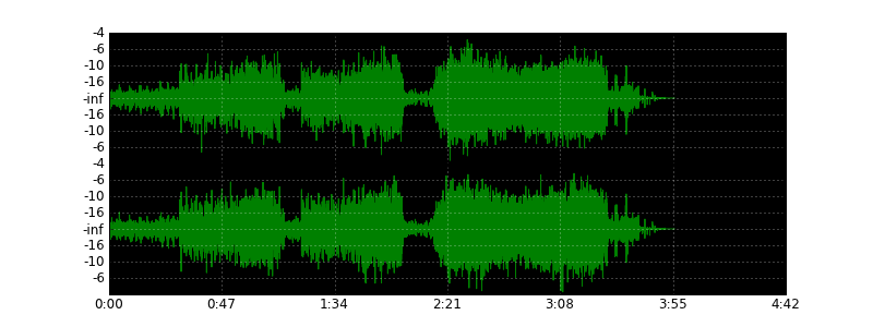
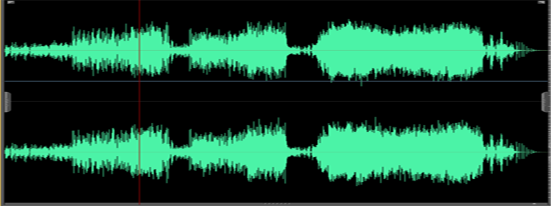
Some time ago I decided to devote myself to solving an exotic task - to draw a wave of a wave file, as audio and video editors do, using Python. As a result, I got a small script that copes with it. So, the picture above is generated by him from the song “Under Pressure” of the Queen group. For comparison - the type of wave in the audio editor:

To parse the sound, I used the numpy library, and for plotting the graph, matplotlib . Under the cat, I lay out the basics of working with wav-files and the script algorithm.

UPD1: thinning coefficient k is better to take approximately k = nframes / w / 32, picked empirically. Updated pictures with a new coefficient.

WAV is a format for storing an uncompressed audio stream, widely used in the media industry. Its peculiarity is that a fixed number of bits are allocated for amplitude coding. This affects the size of the output file, but makes it very easy to read. A typical wave file consists of a header, an audio stream body and a tail for additional information where audio editors can write their own metadata.

The main parameters are extracted from the header part — the number of channels, the bitrate, the number of frames — based on which the audio stream is parsed. The wave file stores 1 or 2 channels, each of which is encoded with 8, 16, 24 or 32 bits. A sequence of bits describing the amplitude of a wave at a point in time is called a sample. The sequence of samples for all channels at a certain moment is called a frame.
')
For example, \ xe2 \ xff \ xe3 \ xf is a frame of a 16-bit wav file. Hence, \ xe2 \ xff is the sample of the first (left) channel, and \ xe3 \ xf is the second (right) channel. Samples are signed integer numbers (except for files with samples of 8 bits, unsigned numbers).

The rich Python library has a wave module designed for parsing wav files. It allows you to get the main characteristics of the sound and read it on separate frames. This is where its capabilities end, and you will have to parse the audio stream yourself.

import wave wav = wave.open("music.wav", mode="r") (nchannels, sampwidth, framerate, nframes, comptype, compname) = wav.getparams() content = wav.readframes(nframes) 

With these lines, we create an object to read the wav file (if the “r” parameter is omitted, then an object will be created for writing that does not suit us). The getparams () method returns a tuple of basic file parameters (in order): the number of channels, the number of bytes per sample, the number of times per second, the total number of frames, the type of compression, the name of the type of compression. I carried them all into separate variables so as not to refer to the fields of the object each time.

The readframes () method reads the specified number of frames relative to the internal pointer of the object and increments it. In this case, we at one time read all the frames in a single byte string into the content variable.

Now we need to parse this line. The sampwidth parameter determines how many bytes are spent on encoding a single sample:

• 1 = 8 bits, unsigned integer (0-255),
• 2 = 16 bits, signed integer (-32768-32767)
• 4 = 32 bits, signed long integer (-2147483648-2147483647)

Parsing is as follows:

 import numpy as np types = { 1: np.int8, 2: np.int16, 4: np.int32 } samples = np.fromstring(content, dtype=types[sampwidth]) 

This is where the numpy library is involved. Its main purpose is mathematical operations with arrays and matrices. Numpy operates with its own data types. The fromstring () function creates a one-dimensional array from a byte string, and the dtype parameter determines how the elements of the array will be interpreted. In our example, the data type is taken from the “types” dictionary, in which the sample sizes and numpy data types are compared.

Now we have an array of audio stream samples. If there is one channel in it, the whole array will represent it, if two (or several), then you need to “thin out” the array by selecting for each channel the kadzh n-th element:

 for n in range(nchannels): channel = samples[n::nchannels] 

In this loop, each audio channel is selected in the channel array using a slice of the form [offset :: n], where offset is the index of the first element and n is the sampling step. But the channel array contains a huge number of points, and the output of the graph for a 3-minute file will require a huge investment of memory and time. Let's enter some additional variables in the code:

 duration = nframes / framerate w, h = 800, 300 DPI = 72 peak = 256 ** sampwidth / 2 k = nframes/w/32 

duration is the duration of the stream in seconds, w and h are the width and height of the output image, DPI is an arbitrary value needed to convert pixels to inches, peak is the peak value of the sample amplitude, k is the channel thinning factor depending on the image width; matched empirically.

Adjust the display of the graph:

 plt.figure(1, figsize=(float(w)/DPI, float(h)/DPI), dpi=DPI) plt.subplots_adjust(wspace=0, hspace=0) 

Now the cycle with the output channels will look like this:

 for n in range(nchannels): channel = samples[n::nchannels] channel = channel[0::k] if nchannels == 1: channel = channel - peak axes = plt.subplot(2, 1, n+1, axisbg="k") axes.plot(channel, "g") axes.yaxis.set_major_formatter(ticker.FuncFormatter(format_db)) plt.grid(True, color="w") axes.xaxis.set_major_formatter(ticker.NullFormatter()) 

The loop checks for the number of channels. As I said, the 8-bit sound is stored in unsigned integers, so it needs to be normalized, taking away half of the amplitude from each sample.

Finally, set the format of the bottom axis

 axes.xaxis.set_major_formatter(ticker.FuncFormatter(format_time)) 

Let's save the graph in the picture and show it:

 plt.savefig("wave", dpi=DPI) plt.show() 

format_time and format_db are functions for formatting the values ​​of the scales of the axes of the abscissas and ordinates.

format_time formats the time by sample number:

 def format_time(x, pos=None): global duration, nframes, k progress = int(x / float(nframes) * duration * k) mins, secs = divmod(progress, 60) hours, mins = divmod(mins, 60) out = "%d:%02d" % (mins, secs) if hours > 0: out = "%d:" % hours return out 

The format_db function formats the sound volume according to its amplitude:

 def format_db(x, pos=None): if pos == 0: return "" global peak if x == 0: return "-inf" db = 20 * math.log10(abs(x) / float(peak)) return int(db) 

The whole script:

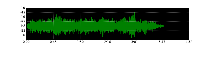
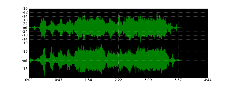
 import wave import numpy as np import matplotlib.pyplot as plt import matplotlib.ticker as ticker import math types = { 1: np.int8, 2: np.int16, 4: np.int32 } def format_time(x, pos=None): global duration, nframes, k progress = int(x / float(nframes) * duration * k) mins, secs = divmod(progress, 60) hours, mins = divmod(mins, 60) out = "%d:%02d" % (mins, secs) if hours > 0: out = "%d:" % hours return out def format_db(x, pos=None): if pos == 0: return "" global peak if x == 0: return "-inf" db = 20 * math.log10(abs(x) / float(peak)) return int(db) wav = wave.open("music.wav", mode="r") (nchannels, sampwidth, framerate, nframes, comptype, compname) = wav.getparams() duration = nframes / framerate w, h = 800, 300 k = nframes/w/32 DPI = 72 peak = 256 ** sampwidth / 2 content = wav.readframes(nframes) samples = np.fromstring(content, dtype=types[sampwidth]) plt.figure(1, figsize=(float(w)/DPI, float(h)/DPI), dpi=DPI) plt.subplots_adjust(wspace=0, hspace=0) for n in range(nchannels): channel = samples[n::nchannels] channel = channel[0::k] if nchannels == 1: channel = channel - peak axes = plt.subplot(2, 1, n+1, axisbg="k") axes.plot(channel, "g") axes.yaxis.set_major_formatter(ticker.FuncFormatter(format_db)) plt.grid(True, color="w") axes.xaxis.set_major_formatter(ticker.NullFormatter()) axes.xaxis.set_major_formatter(ticker.FuncFormatter(format_time)) plt.savefig("wave", dpi=DPI) plt.show() 

More examples: