Implementing graphs and trees in Python
We continue to publish the most interesting chapters from the book Magnus Lie Hetland “Python Algorithms”. The previous article is located at habrahabr.ru/blogs/algorithm/111858 . Today we will discuss the effective work with graphs and trees and the features of their implementation in Python. The basic terminology of graph theory has already been discussed (for example, here: habrahabr.ru/blogs/algorithm/65367 ), so I did not include part of the chapter on terms in this article.
Many tasks, for example, the problem of traversing points along the shortest route, can be solved with the help of one of the most powerful tools - with the help of graphs . Often, if you can determine that you are solving a graph problem, you are at least halfway to a solution. And if your data can somehow be presented as trees , you have every chance to build a truly effective solution.
Any structure or system can be represented as graphs, from the transport network to the data transmission network and from the interaction of proteins in the cell nucleus to connections between people on the Internet.
Your graphs can become even more useful if you add additional data such as weights or distances , which will give an opportunity to describe such various problems as playing chess or determining suitable work for a person according to his abilities.
Trees are just a special kind of graph, so most of the algorithms and graph representations will work for them.
However, due to their special properties (connectedness and absence of cycles), special (and very simple) versions of algorithms and representations can be applied.
In practice, in some cases there are structures (such as XML documents or a directory hierarchy) that can be represented as trees (taking into account the IDREF attributes and symbolic links, XML documents and the directory hierarchy become graphs themselves). In fact, these "some" cases are quite common.
')
The description of the problem in terms of graphs is rather abstract, so if you need to implement a solution, you must provide the graphs in the form of some data structures. (This will have to be done even when designing the algorithm, and only because you need to know how long various operations will be performed on the graph representation). In some cases, the graph will already be compiled in code or data, so a separate structure is not required. For example, if you write a web crawler that collects information about sites by links, the network itself will be the graph. If you have the Person class with the friends attribute, which is a list of other objects of type Person , then your object model will already be a graph on which you can use various algorithms. However, there are special ways to represent graphs.
In general terms, we are looking for a way to implement the adjacency function, N (v) , so that N [v] is some set (or in some cases just an iterator) adjacent to v vertices. As in many other books, we will focus on the two most well-known concepts: adjacency lists and adjacency matrices , because they are most useful and generalized. Alternative views are described in the last section below.
One of the most obvious ways of representing graphs is adjacency lists. Their meaning is that for each vertex there is a list (or a set, or another container or an iterator) of adjacent vertices. Let us analyze the simplest way to implement such a list, assuming that there are n vertices numbered 0 ... n-1 .
Thus, each adjacency list is a list of such numbers, and these lists themselves are assembled into a main list of size n , indexed by vertex numbers. Typically, the sorting of such lists is random, so it really is about using lists to implement adjacency sets . The term list is just historically settled. Python, fortunately, has a separate type for sets, which in many cases is convenient to use.
The approximate graph for which different representations will be shown is shown in fig. 1. To begin with, we assume that all vertices are numbered ( a = 0, b = 1, ... ). With this in mind, the graph can be presented in an obvious way, as shown in the following listing. To make it more convenient, I assigned the numbers of the vertices to variables named according to the vertex marks in the figure. But you can work directly with numbers. Which vertex which list belongs to is indicated in the comments. If you want, take a few minutes to make sure that the presentation matches the picture.
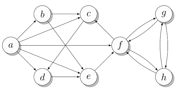
Fig. 1. Approximate graph for the demonstration of different types of presentation
The name N from the listing is associated with the function N described above. In graph theory, N (v) represents a set of vertices adjacent to v . Similarly, in our code, N [v] is a set of vertices adjacent to v . Assuming that N is defined as in the example above, you can study this presentation in interactive Python mode:
Another possible representation, which in some cases gives less overhead, is the adjacency list itself . An example of such a list is shown in the listing below. All the same operations are available, but the vertex adjacency check is performed with Θ (n) . This gives a serious reduction in speed, but if you really need this presentation, then this is his only problem. (If all that your algorithm does is to traverse neighboring vertices, then using objects of the set type is not just pointless: overhead can worsen the constant factors in the asymptotics of your implementation).
It can be argued that this view is in fact a collection of adjacency arrays , not classical adjacency lists , since type list in Python is actually a dynamic array. If you want, you can implement the type of the linked list and use it instead of the type list from Python. This can be done cheaper in terms of performance by arbitrary insertions into the list, but you probably will not need such an operation, because you can just as well add new vertices to the end of the list. The advantage of using the built-in list is that it is a very fast and well-established structure (unlike any list structures that can be implemented in pure Python).
When working with graphs, the idea constantly emerges that the best presentation depends on what exactly needs to be done with the graph. For example, using lists (or arrays) adjacencies can keep the overheads small and provide an efficient N (v) traversal for any vertex v . However, checking whether u and v are contiguous will take time Θ (N (v)) , which can be a problem if the graph is dense (i.e., with a large number of edges). In these cases, come to the aid of many adjacency.
Tip:
It is known that removing objects from the middle of the list in Python is quite expensive. Deletion from the end in this case takes place in constant time. If you do not care about the order of the vertices, you can delete a random vertex for a constant time by overwriting it with the one at the end of the adjacency list, and then calling the pop method.
A small variation on the theme of this view can be called sorted lists of adjacent vertices. If the lists change infrequently, they can be kept sorted and use bisection to check the vertex adjacency, which will lead to a slightly lower overhead (in terms of memory usage and iteration time), but will increase the complexity of the check to (log 2 k) , where k is the number adjacent to this vertex. (This is still a very small value. In practice, however, the use of the built-in type set delivers much less trouble).
Another minor improvement is the use of dictionaries instead of sets or lists. Adjacent vertices can be dictionary keys, and you can use any additional data as a value, for example, the edge weight. How this looks can be seen in the listing below (weights are chosen randomly).
The adjacency dictionary can be used in the same way as other views, taking into account additional information about weights:
If you want, you can use adjacency dictionaries even if you don't have useful data like edge weights (using None or some other value instead of data). This will give you all the advantages of adjacency sets, but it will work with (very, very) old versions of Python that do not have support for the type set (sets were introduced in Python 2.3 as a sets module. The built-in type set is available from Python 2.4).
Up to this point, the entity storing the adjacency structures — lists, sets, or dictionaries — was a list indexed by vertex numbers. A more flexible option (allowing the use of arbitrary, hashable, vertex names) is built on the basis of the dictionary as the main structure (such dictionaries with adjacency lists Guido van Rossum used in his article “Python Patterns - Implementing Graphs” posted at www.python.org /doc/essays/graphs.html ). The listing below shows an example of a dictionary containing adjacency sets. Notice that the vertices in it are indicated by symbols.
If we omit the set constructor from the listing above, then the adjacency lines will remain, which will work as adjacency lists (immutable) of characters (with slightly less overhead). It would seem that this is not a better idea, but, as mentioned above, it all depends on your program. Where do you get the data for the graph? (Maybe they are already in text form?) How are you going to use them?
Another common form of graph representation is adjacency matrices. Their main difference is the following: instead of listing all adjacent vertices, we write one series of values (an array), each of which corresponds to a possible adjacent vertex (there is at least one such for each vertex of the graph), and save the value (in the form of True or False ), indicating whether or not the vertex is adjacent. Again, the simplest implementation can be obtained using nested lists, as can be seen from the listing below. Note that this also requires the vertices to be numbered from 0 to V-1 . Truth values are 1 and 0 (instead of True and False ) to make the matrix readable.
The way to use adjacency matrices is slightly different from lists and adjacency sets. Instead of checking whether b enters N [a] , you will check whether the value of the cell of the matrix N [a] [b] is true. In addition, len (N [a]) can no longer be used to get the number of adjacent vertices, because all rows are of the same length. Instead, you can use the sum function:
The adjacency matrices have a number of useful properties that are worth knowing about. First, since we do not consider graphs with loops (that is, we do not work with pseudographs), all values on the diagonal are false. Also, undirected graphs are usually described by pairs of edges in both directions. This means that the adjacency matrix for an undirected graph will be symmetric.
Expanding the adjacency matrix to use weights is trivial: instead of saving logical values, save weights. In the case of the edge (u, v), N [u] [v] is the weight of the edge w (u, v) instead of True . Often, for practical purposes, non-existent ribs are assigned infinite weights. (This ensures that they will not be included, for example, in the shortest paths, since we are looking for a path along the existing edges). It is not always obvious how to imagine infinity, but there are definitely several different options.
One of them is to use a value that is incorrect for the weight, such as None or -1 , if it is known that all weights are non-negative. It may be useful in some cases to use really large numbers. For integer weights, sys.maxint can be used, although this value is not necessarily the largest (long integers can be larger). There is a value entered to reflect infinity: inf . It is not available in Python directly by name and is expressed as float ('inf') (guaranteed to work for Python 2.6 and later. In earlier versions, these special values were platform-dependent, although float ('inf') or float (' Inf ') should work on most platforms).
The listing below shows how the weights matrix looks like implemented by nested lists. The same weights are used as in the listing above.
The infinite value is indicated by the underscore ( _ ), because it is short and visually distinct. Naturally, you can use any name you prefer. Note that the values on the diagonal are still zero, because even without loops, weights are often interpreted as distances, and the distance from the vertex to itself is zero.
Of course, the weights matrixes make it very easy to get the weights of the edges, but, for example, checking the adjacency and determining the degree of a vertex, or bypassing all adjacent vertices, is done differently. Here you need to use an infinite value, something like this (for greater clarity, we define inf = float ('inf') ):
Note that 1 is subtracted from the degree obtained, because we do not count the values on the diagonal. The complexity of calculating the degree here is Θ (n) , while in another representation both adjacency and the degree of a vertex can be determined in constant time. So you should always understand exactly how you are going to use your graph and choose the appropriate presentation for it.
Any graph representation can naturally be used to represent trees, because trees are a special kind of graph. However, trees play a big role in algorithms, and many corresponding structures and methods have been developed for them. Most algorithms on trees (for example, search in trees) can be viewed in terms of graph theory, but special data structures make them easier to implement.
The easiest way to describe the representation of the tree with the root, in which the edges go down from the root. Such trees often display hierarchical data branching, where the root displays all objects (which may be stored in the leaves), and each internal node shows the objects contained in the tree whose root is this node. This description can be used by presenting each subtree with a list containing all its descendant subtrees. Consider a simple tree shown in the figure. 2
We can present this tree as a list of lists:
Each list is essentially a list of descendants of each of the internal nodes. In the second example, we refer to the third descendant of the root, then its second descendant, and finally the first descendant of the previous node (this path is marked in the figure).

Fig. 2. An example of a tree with a marked path from root to leaf
In some cases it is possible to pre-determine the maximum number of descendants of each node. (For example, each node of a binary tree can have up to two children). Therefore, you can use other representations, for example, objects with a separate attribute for each of the descendants as in the listing below.
You can use None to indicate missing descendants (if the node has only one descendant). Of course, you can combine different methods (for example, using lists or sets of descendants for each node).
A common way to implement trees, especially in languages that do not have built-in support for lists, is the so-called “first descendant, next brother” representation. In it, each node has two “pointers” or attributes pointing to other nodes, as in a binary tree. However, the first of these attributes refers to the first descendant of the node, and the second to its next brother (i.e., a node that has the same parent but is to the right, approx. Transl .). In other words, each tree node has a pointer to a linked list of its descendants, and each of these descendants refers to its own similar list. Thus, a small modification of the binary tree will give us the multipath tree shown in the listing below.
A separate attribute val is introduced here simply to get a clear conclusion when specifying a value (for example, “c”) instead of a link to a node. Naturally, all this can be changed. Here is an example of how to handle this structure:
This is how the tree looks like:

The attributes kids and next are shown with dashed lines, and the edges of the tree themselves are solid. I cheated a little and did not show separate nodes for the lines “a”, “b”, etc. Instead, I treat them as tags on the respective parent nodes. In a more complex tree, instead of using a single attribute to store the value of a node and to reference a list of descendants, you might need separate attributes for both purposes. Typically, a more complex code (including loops and recursion) is used to bypass the tree than is given here with a fixed path.
Despite the fact that there are many representations of graphs, most study and use only two types (with modifications) already described in this chapter. Jeremy Spinred writes in his book “Effective Graph Representation” that he, as a researcher of computer representation of graphs, is “particularly annoyed” by most introductory articles. The descriptions in them of well-known representations (lists and adjacency matrices) are usually adequate, but more general explanations are often erroneous. , :
« : . , , , , , » (. 9).
, . -, , . , ( ), ( -), , , ( ). , ( ) ( ). , , - .
-, : , , , , .
, , , , . , , , . , (u, v) Θ(1) , v — Θ(n) , Θ(d(v)) , .. .
If the asymptotic complexity of your algorithm does not depend on the type of representation, you can conduct any empirical tests described earlier in this chapter. Or, as often happens, you can choose a view that fits better with your code and is easier to maintain.
An important way to use graphs, which has not yet been affected, does not concern their presentation. The fact is that in many problems the data already has a graph structure, or even a tree, and we can use appropriate algorithms for them for graphs and trees without creating special representations. In some cases this happens if the graph representation is made outside of our program. For example, when parsing XML documents or traversing file system directories, a tree structure has already been created and there are certain APIs for it. In other words, we implicitly define a graph. For example, to find the most effective solution for a given configuration of the Rubik's cube, you can determine the state of the cube and methods for changing it. But even if you do not explicitly describe and save each configuration,possible states will form an implicit graph (or a set of vertices) with edges - state change operators. Next, you can use algorithms such as A * or Dijkstra's bidirectional algorithm to find the shortest path to the solution state. In such cases, the function of obtaining neighboring vertices N (v) will work on the fly, probably returning adjacent vertices as a collection or other form of an iterator object.
And the last type of graphs, which I will touch on in this chapter, is called a subtask graph . This is a deep concept, to which I will repeatedly refer to, describing various techniques for constructing algorithms. In short, most tasks can be decomposed into subtasks. : , . , (.. ) . ( ), « » .
, , , . , , , . , C, . , . , :
NetworkX: http://networkx.lanl.gov
python-graph: http://code.google.com/p/python-graph
Graphine: http://gitorious.org/projects/graphine/pages/Home
, Pygr, ( http://bioinfo.mbi.ucla.edu/pygr ), Gato, ( http://gato.sourceforge.net ) PADS, ( http://www.ics.uci.edu/~eppstein/PADS ).
Implementing graphs and trees
Many tasks, for example, the problem of traversing points along the shortest route, can be solved with the help of one of the most powerful tools - with the help of graphs . Often, if you can determine that you are solving a graph problem, you are at least halfway to a solution. And if your data can somehow be presented as trees , you have every chance to build a truly effective solution.
Any structure or system can be represented as graphs, from the transport network to the data transmission network and from the interaction of proteins in the cell nucleus to connections between people on the Internet.
Your graphs can become even more useful if you add additional data such as weights or distances , which will give an opportunity to describe such various problems as playing chess or determining suitable work for a person according to his abilities.
Trees are just a special kind of graph, so most of the algorithms and graph representations will work for them.
However, due to their special properties (connectedness and absence of cycles), special (and very simple) versions of algorithms and representations can be applied.
In practice, in some cases there are structures (such as XML documents or a directory hierarchy) that can be represented as trees (taking into account the IDREF attributes and symbolic links, XML documents and the directory hierarchy become graphs themselves). In fact, these "some" cases are quite common.
')
The description of the problem in terms of graphs is rather abstract, so if you need to implement a solution, you must provide the graphs in the form of some data structures. (This will have to be done even when designing the algorithm, and only because you need to know how long various operations will be performed on the graph representation). In some cases, the graph will already be compiled in code or data, so a separate structure is not required. For example, if you write a web crawler that collects information about sites by links, the network itself will be the graph. If you have the Person class with the friends attribute, which is a list of other objects of type Person , then your object model will already be a graph on which you can use various algorithms. However, there are special ways to represent graphs.
In general terms, we are looking for a way to implement the adjacency function, N (v) , so that N [v] is some set (or in some cases just an iterator) adjacent to v vertices. As in many other books, we will focus on the two most well-known concepts: adjacency lists and adjacency matrices , because they are most useful and generalized. Alternative views are described in the last section below.
"Black Box": dictionaries and sets
, , Python, — <em></em>. ( ), . , , ( , ). Python hash: >>> hash(42) 42 >>> hash("Hello, world!") -1886531940 , -. . , ( -, ). , Θ(1). ( Θ(n), -. , ). , dict set , . Connectivity lists and the like
One of the most obvious ways of representing graphs is adjacency lists. Their meaning is that for each vertex there is a list (or a set, or another container or an iterator) of adjacent vertices. Let us analyze the simplest way to implement such a list, assuming that there are n vertices numbered 0 ... n-1 .
, . 0… n-1 , . Thus, each adjacency list is a list of such numbers, and these lists themselves are assembled into a main list of size n , indexed by vertex numbers. Typically, the sorting of such lists is random, so it really is about using lists to implement adjacency sets . The term list is just historically settled. Python, fortunately, has a separate type for sets, which in many cases is convenient to use.
The approximate graph for which different representations will be shown is shown in fig. 1. To begin with, we assume that all vertices are numbered ( a = 0, b = 1, ... ). With this in mind, the graph can be presented in an obvious way, as shown in the following listing. To make it more convenient, I assigned the numbers of the vertices to variables named according to the vertex marks in the figure. But you can work directly with numbers. Which vertex which list belongs to is indicated in the comments. If you want, take a few minutes to make sure that the presentation matches the picture.
a, b, c, d, e, f, g, h = range(8) N = [ {b, c, d, e, f}, # a {c, e}, # b {d}, # c {e}, # d {f}, # e {c, g, h}, # f {f, h}, # g {f, g} # h ] Python 2.7 ( 3.0) set([1, 2, 3]) {1, 2, 3}. - set(), {} . Fig. 1. Approximate graph for the demonstration of different types of presentation
The name N from the listing is associated with the function N described above. In graph theory, N (v) represents a set of vertices adjacent to v . Similarly, in our code, N [v] is a set of vertices adjacent to v . Assuming that N is defined as in the example above, you can study this presentation in interactive Python mode:
>>> b in N[a] # ? True >>> len(N[f]) # 3 : , , , , , python -i, : python -i listing_2_1.py , , , . Another possible representation, which in some cases gives less overhead, is the adjacency list itself . An example of such a list is shown in the listing below. All the same operations are available, but the vertex adjacency check is performed with Θ (n) . This gives a serious reduction in speed, but if you really need this presentation, then this is his only problem. (If all that your algorithm does is to traverse neighboring vertices, then using objects of the set type is not just pointless: overhead can worsen the constant factors in the asymptotics of your implementation).
a, b, c, d, e, f, g, h = range(8) N = [ [b, c, d, e, f], # a [c, e], # b [d], # c [e], # d [f], # e [c, g, h], # f [f, h], # g [f, g] # h ] It can be argued that this view is in fact a collection of adjacency arrays , not classical adjacency lists , since type list in Python is actually a dynamic array. If you want, you can implement the type of the linked list and use it instead of the type list from Python. This can be done cheaper in terms of performance by arbitrary insertions into the list, but you probably will not need such an operation, because you can just as well add new vertices to the end of the list. The advantage of using the built-in list is that it is a very fast and well-established structure (unlike any list structures that can be implemented in pure Python).
When working with graphs, the idea constantly emerges that the best presentation depends on what exactly needs to be done with the graph. For example, using lists (or arrays) adjacencies can keep the overheads small and provide an efficient N (v) traversal for any vertex v . However, checking whether u and v are contiguous will take time Θ (N (v)) , which can be a problem if the graph is dense (i.e., with a large number of edges). In these cases, come to the aid of many adjacency.
Tip:
It is known that removing objects from the middle of the list in Python is quite expensive. Deletion from the end in this case takes place in constant time. If you do not care about the order of the vertices, you can delete a random vertex for a constant time by overwriting it with the one at the end of the adjacency list, and then calling the pop method.
A small variation on the theme of this view can be called sorted lists of adjacent vertices. If the lists change infrequently, they can be kept sorted and use bisection to check the vertex adjacency, which will lead to a slightly lower overhead (in terms of memory usage and iteration time), but will increase the complexity of the check to (log 2 k) , where k is the number adjacent to this vertex. (This is still a very small value. In practice, however, the use of the built-in type set delivers much less trouble).
Another minor improvement is the use of dictionaries instead of sets or lists. Adjacent vertices can be dictionary keys, and you can use any additional data as a value, for example, the edge weight. How this looks can be seen in the listing below (weights are chosen randomly).
a, b, c, d, e, f, g, h = range(8) N = [ {b:2, c:1, d:3, e:9, f:4}, # a {c:4, e:3}, # b {d:8}, # c {e:7}, # d {f:5}, # e {c:2, g:2, h:2}, # f {f:1, h:6}, # g {f:9, g:8} # h ] The adjacency dictionary can be used in the same way as other views, taking into account additional information about weights:
>>> b in N[a] # True >>> len(N[f]) # 3 >>> N[a][b] # (a, b) 2 If you want, you can use adjacency dictionaries even if you don't have useful data like edge weights (using None or some other value instead of data). This will give you all the advantages of adjacency sets, but it will work with (very, very) old versions of Python that do not have support for the type set (sets were introduced in Python 2.3 as a sets module. The built-in type set is available from Python 2.4).
Up to this point, the entity storing the adjacency structures — lists, sets, or dictionaries — was a list indexed by vertex numbers. A more flexible option (allowing the use of arbitrary, hashable, vertex names) is built on the basis of the dictionary as the main structure (such dictionaries with adjacency lists Guido van Rossum used in his article “Python Patterns - Implementing Graphs” posted at www.python.org /doc/essays/graphs.html ). The listing below shows an example of a dictionary containing adjacency sets. Notice that the vertices in it are indicated by symbols.
N = { 'a': set('bcdef'), 'b': set('ce'), 'c': set('d'), 'd': set('e'), 'e': set('f'), 'f': set('cgh'), 'g': set('fh'), 'h': set('fg') } If we omit the set constructor from the listing above, then the adjacency lines will remain, which will work as adjacency lists (immutable) of characters (with slightly less overhead). It would seem that this is not a better idea, but, as mentioned above, it all depends on your program. Where do you get the data for the graph? (Maybe they are already in text form?) How are you going to use them?
Adjacency matrices
Another common form of graph representation is adjacency matrices. Their main difference is the following: instead of listing all adjacent vertices, we write one series of values (an array), each of which corresponds to a possible adjacent vertex (there is at least one such for each vertex of the graph), and save the value (in the form of True or False ), indicating whether or not the vertex is adjacent. Again, the simplest implementation can be obtained using nested lists, as can be seen from the listing below. Note that this also requires the vertices to be numbered from 0 to V-1 . Truth values are 1 and 0 (instead of True and False ) to make the matrix readable.
a, b, c, d, e, f, g, h = range(8) # abcdefgh N = [[0,1,1,1,1,1,0,0], # a [0,0,1,0,1,0,0,0], # b [0,0,0,1,0,0,0,0], # c [0,0,0,0,1,0,0,0], # d [0,0,0,0,0,1,0,0], # e [0,0,1,0,0,0,1,1], # f [0,0,0,0,0,1,0,1], # g [0,0,0,0,0,1,1,0]] # h The way to use adjacency matrices is slightly different from lists and adjacency sets. Instead of checking whether b enters N [a] , you will check whether the value of the cell of the matrix N [a] [b] is true. In addition, len (N [a]) can no longer be used to get the number of adjacent vertices, because all rows are of the same length. Instead, you can use the sum function:
>>> N[a][b] 1 >>> sum(N[f]) 3 The adjacency matrices have a number of useful properties that are worth knowing about. First, since we do not consider graphs with loops (that is, we do not work with pseudographs), all values on the diagonal are false. Also, undirected graphs are usually described by pairs of edges in both directions. This means that the adjacency matrix for an undirected graph will be symmetric.
Expanding the adjacency matrix to use weights is trivial: instead of saving logical values, save weights. In the case of the edge (u, v), N [u] [v] is the weight of the edge w (u, v) instead of True . Often, for practical purposes, non-existent ribs are assigned infinite weights. (This ensures that they will not be included, for example, in the shortest paths, since we are looking for a path along the existing edges). It is not always obvious how to imagine infinity, but there are definitely several different options.
One of them is to use a value that is incorrect for the weight, such as None or -1 , if it is known that all weights are non-negative. It may be useful in some cases to use really large numbers. For integer weights, sys.maxint can be used, although this value is not necessarily the largest (long integers can be larger). There is a value entered to reflect infinity: inf . It is not available in Python directly by name and is expressed as float ('inf') (guaranteed to work for Python 2.6 and later. In earlier versions, these special values were platform-dependent, although float ('inf') or float (' Inf ') should work on most platforms).
The listing below shows how the weights matrix looks like implemented by nested lists. The same weights are used as in the listing above.
a, b, c, d, e, f, g, h = range(8) _ = float('inf') # abcdefgh W = [[0,2,1,3,9,4,_,_], # a [_,0,4,_,3,_,_,_], # b [_,_,0,8,_,_,_,_], # c [_,_,_,0,7,_,_,_], # d [_,_,_,_,0,5,_,_], # e [_,_,2,_,_,0,2,2], # f [_,_,_,_,_,1,0,6], # g [_,_,_,_,_,9,8,0]] # h The infinite value is indicated by the underscore ( _ ), because it is short and visually distinct. Naturally, you can use any name you prefer. Note that the values on the diagonal are still zero, because even without loops, weights are often interpreted as distances, and the distance from the vertex to itself is zero.
Of course, the weights matrixes make it very easy to get the weights of the edges, but, for example, checking the adjacency and determining the degree of a vertex, or bypassing all adjacent vertices, is done differently. Here you need to use an infinite value, something like this (for greater clarity, we define inf = float ('inf') ):
>>> W[a][b] < inf # True >>> W[c][e] < inf # False >>> sum(1 for w in W[a] if w < inf) - 1 # 5 Note that 1 is subtracted from the degree obtained, because we do not count the values on the diagonal. The complexity of calculating the degree here is Θ (n) , while in another representation both adjacency and the degree of a vertex can be determined in constant time. So you should always understand exactly how you are going to use your graph and choose the appropriate presentation for it.
NumPy special purpose arrays
NumPy , . , NumPy , , . n , : >>> N = [[0]*10 for i in range(10)] NumPy zeros: >>> import numpy as np >>> N = np.zeros([10,10]) , : A[u,v]. , : A[u]. NumPy http://numpy.scipy.org. , NumPy, Python. NumPy Python, , . (, Subversion): svn co http://svn.scipy.org/svn/numpy/trunk numpy , NumPy, , . Implementation of trees
Any graph representation can naturally be used to represent trees, because trees are a special kind of graph. However, trees play a big role in algorithms, and many corresponding structures and methods have been developed for them. Most algorithms on trees (for example, search in trees) can be viewed in terms of graph theory, but special data structures make them easier to implement.
The easiest way to describe the representation of the tree with the root, in which the edges go down from the root. Such trees often display hierarchical data branching, where the root displays all objects (which may be stored in the leaves), and each internal node shows the objects contained in the tree whose root is this node. This description can be used by presenting each subtree with a list containing all its descendant subtrees. Consider a simple tree shown in the figure. 2
We can present this tree as a list of lists:
>>> T = [["a", "b"], ["c"], ["d", ["e", "f"]]] >>> T[0][1] 'b' >>> T[2][1][0] 'e' Each list is essentially a list of descendants of each of the internal nodes. In the second example, we refer to the third descendant of the root, then its second descendant, and finally the first descendant of the previous node (this path is marked in the figure).
Fig. 2. An example of a tree with a marked path from root to leaf
In some cases it is possible to pre-determine the maximum number of descendants of each node. (For example, each node of a binary tree can have up to two children). Therefore, you can use other representations, for example, objects with a separate attribute for each of the descendants as in the listing below.
class Tree: def __init__(self, left, right): self.left = left self.right = right >>> t = Tree(Tree("a", "b"), Tree("c", "d")) >>> t.right.left 'c' You can use None to indicate missing descendants (if the node has only one descendant). Of course, you can combine different methods (for example, using lists or sets of descendants for each node).
A common way to implement trees, especially in languages that do not have built-in support for lists, is the so-called “first descendant, next brother” representation. In it, each node has two “pointers” or attributes pointing to other nodes, as in a binary tree. However, the first of these attributes refers to the first descendant of the node, and the second to its next brother (i.e., a node that has the same parent but is to the right, approx. Transl .). In other words, each tree node has a pointer to a linked list of its descendants, and each of these descendants refers to its own similar list. Thus, a small modification of the binary tree will give us the multipath tree shown in the listing below.
class Tree: def __init__(self, kids, next=None): self.kids = self.val = kids self.next = next A separate attribute val is introduced here simply to get a clear conclusion when specifying a value (for example, “c”) instead of a link to a node. Naturally, all this can be changed. Here is an example of how to handle this structure:
>>> t = Tree(Tree("a", Tree("b", Tree("c", Tree("d"))))) >>> t.kids.next.next.val 'c' This is how the tree looks like:
The attributes kids and next are shown with dashed lines, and the edges of the tree themselves are solid. I cheated a little and did not show separate nodes for the lines “a”, “b”, etc. Instead, I treat them as tags on the respective parent nodes. In a more complex tree, instead of using a single attribute to store the value of a node and to reference a list of descendants, you might need separate attributes for both purposes. Typically, a more complex code (including loops and recursion) is used to bypass the tree than is given here with a fixed path.
Set Design Pattern
( ) , . «» ( «Python Cookbook»). , : class Bunch(dict): def __init__(self, *args, **kwds): super(Bunch, self).__init__(*args, **kwds) self.__dict__ = self . -, , : >>> x = Bunch(name="Jayne Cobb", position="PR") >>> x.name 'Jayne Cobb' -, dict , () . : >>> T = Bunch >>> t = T(left=T(left="a", right="b"), right=T(left="c")) >>> t.left {'right': 'b', 'left': 'a'} >>> t.left.right 'b' >>> t['left']['right'] 'b' >>> "left" in t.right True >>> "right" in t.right False . , , . Many different views
Despite the fact that there are many representations of graphs, most study and use only two types (with modifications) already described in this chapter. Jeremy Spinred writes in his book “Effective Graph Representation” that he, as a researcher of computer representation of graphs, is “particularly annoyed” by most introductory articles. The descriptions in them of well-known representations (lists and adjacency matrices) are usually adequate, but more general explanations are often erroneous. , :
« : . , , , , , » (. 9).
, . -, , . , ( ), ( -), , , ( ). , ( ) ( ). , , - .
-, : , , , , .
, , , , . , , , . , (u, v) Θ(1) , v — Θ(n) , Θ(d(v)) , .. .
If the asymptotic complexity of your algorithm does not depend on the type of representation, you can conduct any empirical tests described earlier in this chapter. Or, as often happens, you can choose a view that fits better with your code and is easier to maintain.
An important way to use graphs, which has not yet been affected, does not concern their presentation. The fact is that in many problems the data already has a graph structure, or even a tree, and we can use appropriate algorithms for them for graphs and trees without creating special representations. In some cases this happens if the graph representation is made outside of our program. For example, when parsing XML documents or traversing file system directories, a tree structure has already been created and there are certain APIs for it. In other words, we implicitly define a graph. For example, to find the most effective solution for a given configuration of the Rubik's cube, you can determine the state of the cube and methods for changing it. But even if you do not explicitly describe and save each configuration,possible states will form an implicit graph (or a set of vertices) with edges - state change operators. Next, you can use algorithms such as A * or Dijkstra's bidirectional algorithm to find the shortest path to the solution state. In such cases, the function of obtaining neighboring vertices N (v) will work on the fly, probably returning adjacent vertices as a collection or other form of an iterator object.
And the last type of graphs, which I will touch on in this chapter, is called a subtask graph . This is a deep concept, to which I will repeatedly refer to, describing various techniques for constructing algorithms. In short, most tasks can be decomposed into subtasks. : , . , (.. ) . ( ), « » .
, , , . , , , . , C, . , . , :
NetworkX: http://networkx.lanl.gov
python-graph: http://code.google.com/p/python-graph
Graphine: http://gitorious.org/projects/graphine/pages/Home
, Pygr, ( http://bioinfo.mbi.ucla.edu/pygr ), Gato, ( http://gato.sourceforge.net ) PADS, ( http://www.ics.uci.edu/~eppstein/PADS ).
Source: https://habr.com/ru/post/112421/
All Articles