MATLAB and fast Fourier transform
At work, I repeatedly encountered the need to quickly determine the presence of harmonic components in the signal. Often, for an approximate assessment, it is sufficient to use the fast Fourier transform algorithm. Moreover, its implementation is available in almost all mathematical packages and libraries, and it will not be difficult to implement it yourself. Meanwhile, experience shows that, for all its simplicity, the method begins to raise some questions when it becomes necessary not only to look for the presence of discretes in the signal, but also to find out their absolute values, i.e. normalize the result.
In this article I will try to explain what the fft (Fast Fourier transform) gives as a result using the example of MATLAB (and as a bonus I will spend a small educational program on this very useful, in my opinion, language).
MATLAB allows you to not bother with the manual removal of unnecessary objects, however, when working with more or less voluminous data sets, it has a habit of being capricious and complaining about the lack of memory. To clear the memory, use the clear procedure with the name of the object to be deleted.
Let's start with this. Since we will generate everything we need on our own, we can safely delete everything that has accumulated in the workspace during an active session, simply by adding the all keyword:
')
So, first of all, let's set the initial data for our model. Fourier analysis is ideal for isolating harmonic signals against interference. In order to demonstrate this, we take as the signal the sum of some constant and two sinusoids with different frequency and amplitude. We take the noise dispersion 3 times the amplitude of the first sinusoid. We will also set the number of frequency bands that the fft algorithm should calculate. A semicolon at the end of lines is not necessary, and if you do not put it, the result of calculating functions and setting variables will be duplicated into the command line, which can be used to debug the code (however, 512 values with a solid canvas in the command line are unlikely to help you, especially that their output also takes a certain amount of time, so it is still better to remember to close the lines).
MATLAB (Matrix Laboratory), as the name implies, is designed primarily for working with arrays, almost all of the algorithms of counting in it are optimized for working with vectors. The abundance of convenient tools of work also unobtrusively pushes to present as much as possible of the initial data in the form of matrices. In particular, it is easy to generate an array of increasing (decreasing) values with a given step (1 \ Fd in this example):
Random Gaussian noise is given by the randn function, the result of which is an array of the dimension specified in its parameters. For consistency, we set it as a string (first parameter 1) with a length corresponding to the length of our array of time samples, which in turn is calculated by the function length.
The * symbol is used to mean multiplication. Because most often actions are performed on vectors, then multiplication is implied to be vectorial, but you can also easily, without overloading this operator, use it for elementwise multiplication, adding a period (. *) in front of it. When multiplying a vector by a scalar, a dot before multiplication is not mandatory. Also the added point will make elementwise exponentiation and division.
We now turn to that for the sake of which this article was started - functions fft (). The arguments of the standard MATLAB function are the signal itself (in our case, Signal), the dimension of the result vector (FftL), and measurement.
The last argument determines along which dimension the signal is located if a multidimensional array is input (Sometimes this parameter is mistaken for the Fourier transform dimension, but it is not. Although MATLAB has implementations of 2-dimensional fft2 () and multidimensional fftn () algorithms) . Since our signal is a vector, it is quite possible to omit it.
Consider first the signal without the admixture of noise. As a result, we get the vector of complex numbers. This is the representation of our signal in the frequency domain in exponential form. Those. the modules of these complex numbers represent the amplitudes of the corresponding frequencies (more precisely, the frequency bands, see further), and the arguments are their initial phases. And if the obtained phase is uniquely calculated in radians, then with amplitude and frequencies it is not so simple.
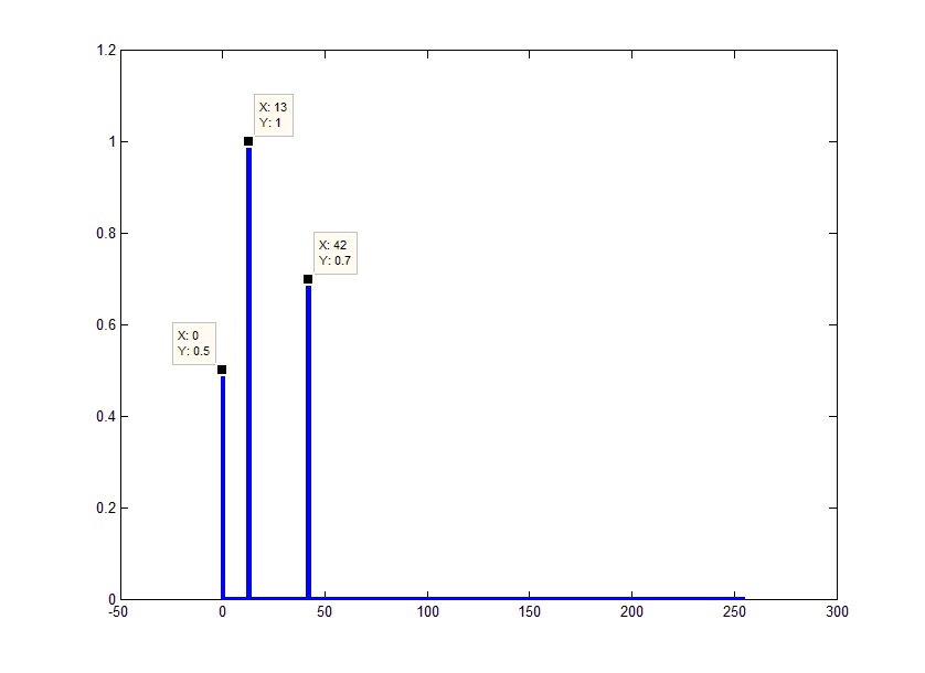
For example, if we simply apply the Fourier transform to our signal, and take the absolute values of the output vector, we get approximately the following image:
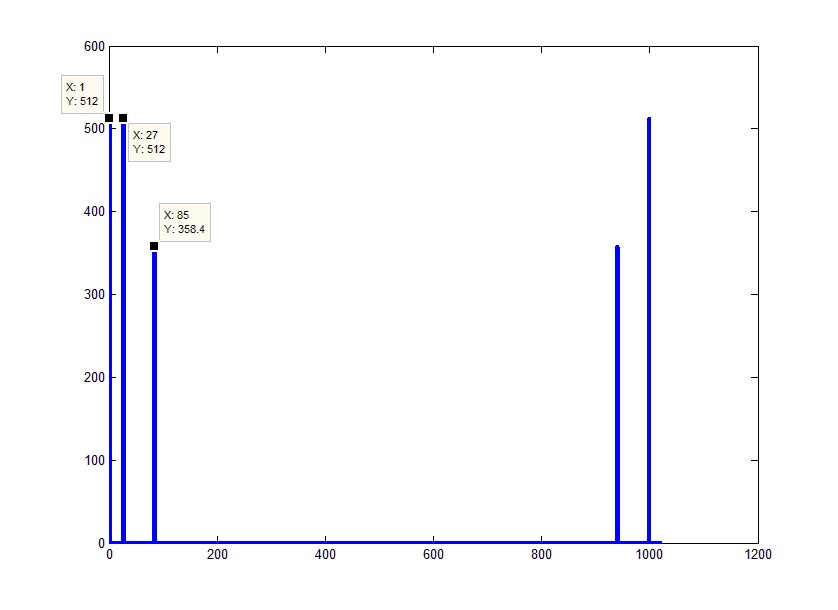
To construct two-dimensional graphs, it is convenient to use the function plot. The main parameters used in this function are one-dimensional arrays of points, the first specifies the axis of ordinates, the second the value of the function at the corresponding points. If you pass only one array, it will be displayed with a fixed step of 1.
If you look at the resulting picture, it turns out that it is somewhat different from our expectations. In the above graph, 5 peaks instead of the expected 3x (constant + 2 sinusoids), their amplitudes do not coincide with the amplitudes of the original signals, and the abscissa axis hardly represents the frequencies.
First of all, it should be taken into account that the counting of the algorithm is arranged in such a way that not only positive, but also negative frequencies get over and the right part of the graph is a “mirror” display of the real spectrum. Those. in fact, 0 (to which the constant part of the signal corresponds) must fall in the middle of the array. The situation can be corrected by making a cyclic shift half the length of the array. For these purposes, in MATLAB, there is a shift function fftshift (), which displaces the first element in the middle of the array:
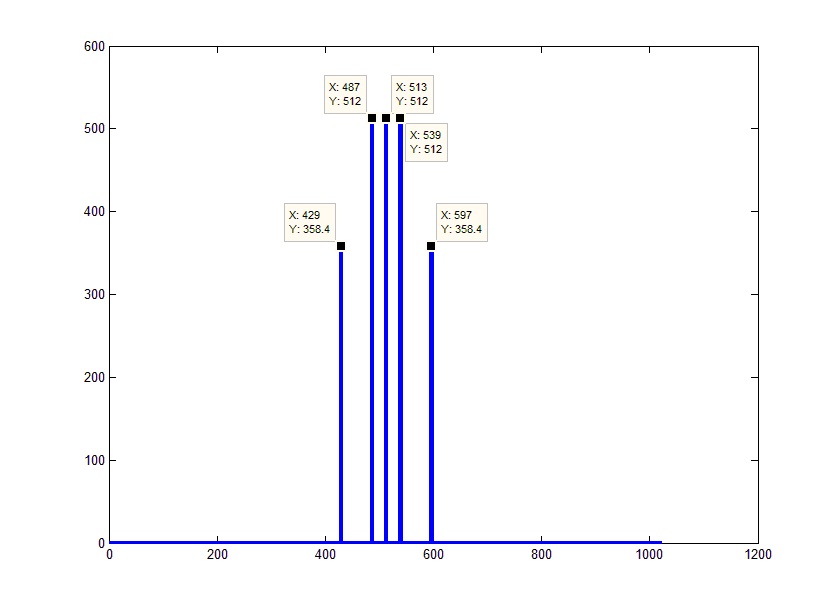
Now pay attention to the axis of values.
According to the sampling theorem (also known as the Nyquist-Shannon theorem or more patriotic Kotelnikov theorem), the spectrum of a discrete signal will be limited to half the sampling rate (Fd). Or in our case, –Fd / 2 on the left and Fd / 2 on the right. Those. all received array covers Fd frequencies. From here, given that we know (or rather, even independently set as a parameter) the length of the array, we obtain frequencies as an array of values from –Fd / 2 to Fd / 2 with a step Fd / FftL (in fact, the rightmost frequency will be less than one border countdown ie Fd / 2-Fd / FftL):
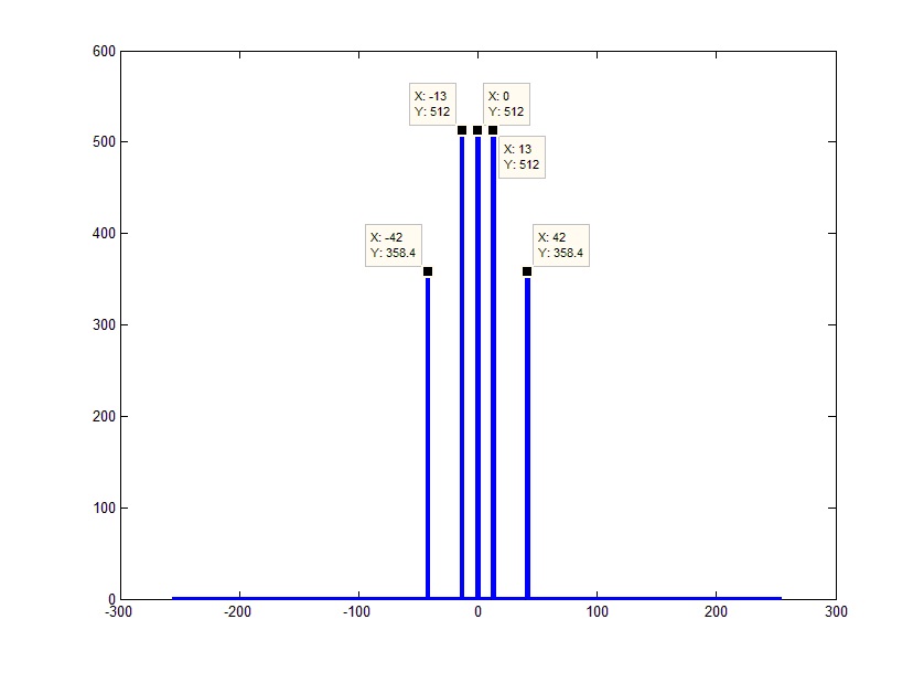
If you look at the phase of the frequencies, you can see that they are equal to the negative phases of the corresponding negative frequencies. Given the equality of the amplitudes of the left and right sides of the spectrum and the correspondence of their phases to within a sign, the whole spectrum will be equivalent to its positive part with a double amplitude. The only exception is 0 element, which does not have a mirror half. Thus, you can get rid of the "incomprehensible" and often unnecessary negative frequencies. This could be done right away simply by discarding the end of the original array and multiplying the remaining elements by 2 (except for the constant component):
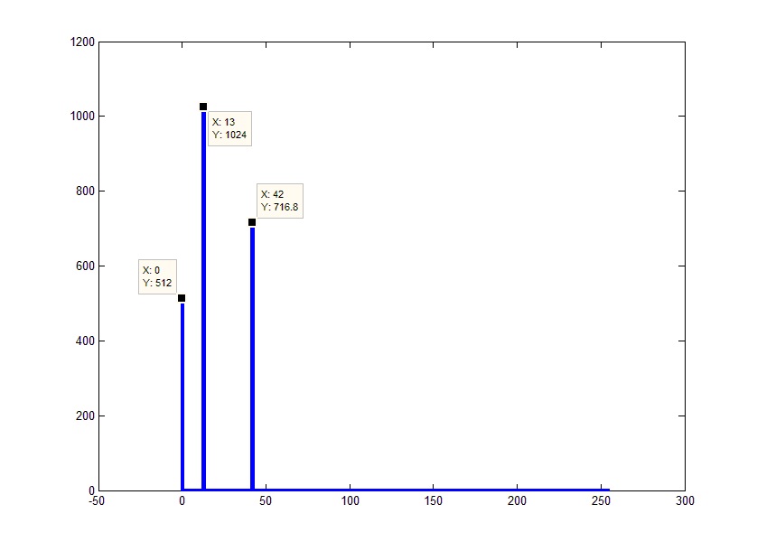
Now it looks like the result we expect. The only thing that confuses now is the amplitudes. With this, everything is quite simple. Because Since the fast Fourier transform is actually a summation of the signal multiplied by the core of the transform (complex exponential) for each of the frequencies, the actual result will be less than that obtained exactly in the number of summations (frequencies as a result), i.e. the result must be divided into the number of elements in the result (do not forget that the result is the entire answer, together with the rejected part, that is, our given FftL):
Another thing worth mentioning. In the spectral representation, the signal is calculated not at the frequency at which the algorithm hit (as we remember, the frequencies follow with the Fd / FftL step), but the value in the band (the width is equal to the step). Those. if several discretes fall into this band, they are added together. For example, you can reduce the number of lines as a result of the algorithm:
However, this does not mean that it is worthless to immediately increase the accuracy of work, since This also leads to negative consequences, because If the resolution is comparable to the sampling rate of a signal, the harmonics of the “window” will enter the spectrum, which are related not to the real signal, but to its discrete representation:
Or closer to one of the discrete neighborhoods:
The code for normalizing fft will look something like this:
We only need to display the results. The subplot function allows you to split the window into several areas to display graphs.
The result of the code will be as follows:
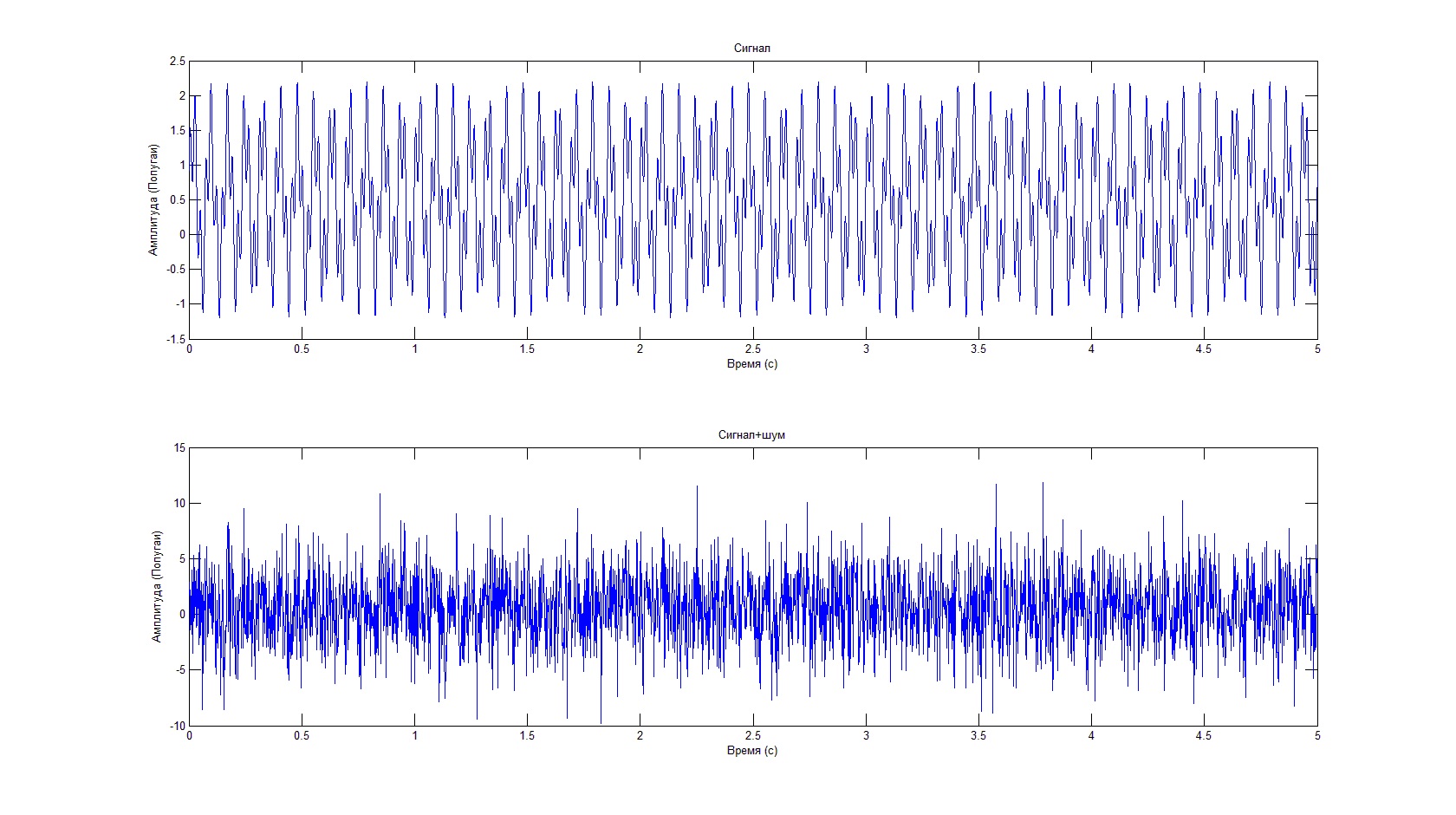
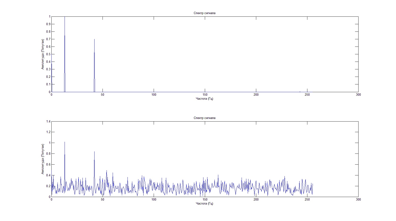
Despite the fact that the useful signal is not visible against the background of noise, the spectral characteristic allows us to determine its frequency and amplitude.
I hope this text was useful to you.
In this article I will try to explain what the fft (Fast Fourier transform) gives as a result using the example of MATLAB (and as a bonus I will spend a small educational program on this very useful, in my opinion, language).
MATLAB allows you to not bother with the manual removal of unnecessary objects, however, when working with more or less voluminous data sets, it has a habit of being capricious and complaining about the lack of memory. To clear the memory, use the clear procedure with the name of the object to be deleted.
Let's start with this. Since we will generate everything we need on our own, we can safely delete everything that has accumulated in the workspace during an active session, simply by adding the all keyword:
')
clear all%So, first of all, let's set the initial data for our model. Fourier analysis is ideal for isolating harmonic signals against interference. In order to demonstrate this, we take as the signal the sum of some constant and two sinusoids with different frequency and amplitude. We take the noise dispersion 3 times the amplitude of the first sinusoid. We will also set the number of frequency bands that the fft algorithm should calculate. A semicolon at the end of lines is not necessary, and if you do not put it, the result of calculating functions and setting variables will be duplicated into the command line, which can be used to debug the code (however, 512 values with a solid canvas in the command line are unlikely to help you, especially that their output also takes a certain amount of time, so it is still better to remember to close the lines).
%%
Tm=5;% ()
Fd=512;% ()
Ak=0.5;% ()
A1=1;% ()
A2=0.7;% ()
F1=13;% ()
F2=42;% ()
Phi1=0;% ()
Phi2=37;% ()
An=3*A1;% ()
FftL=1024;%
MATLAB (Matrix Laboratory), as the name implies, is designed primarily for working with arrays, almost all of the algorithms of counting in it are optimized for working with vectors. The abundance of convenient tools of work also unobtrusively pushes to present as much as possible of the initial data in the form of matrices. In particular, it is easy to generate an array of increasing (decreasing) values with a given step (1 \ Fd in this example):
%%
T=0:1/Fd:Tm;%
Random Gaussian noise is given by the randn function, the result of which is an array of the dimension specified in its parameters. For consistency, we set it as a string (first parameter 1) with a length corresponding to the length of our array of time samples, which in turn is calculated by the function length.
Noise=An*randn(1,length(T));%The * symbol is used to mean multiplication. Because most often actions are performed on vectors, then multiplication is implied to be vectorial, but you can also easily, without overloading this operator, use it for elementwise multiplication, adding a period (. *) in front of it. When multiplying a vector by a scalar, a dot before multiplication is not mandatory. Also the added point will make elementwise exponentiation and division.
Signal=Ak+A1*sind((F1*360).*T+Phi1)+A2*sind((F2*360).*T+Phi2);% ( 2 )We now turn to that for the sake of which this article was started - functions fft (). The arguments of the standard MATLAB function are the signal itself (in our case, Signal), the dimension of the result vector (FftL), and measurement.
The last argument determines along which dimension the signal is located if a multidimensional array is input (Sometimes this parameter is mistaken for the Fourier transform dimension, but it is not. Although MATLAB has implementations of 2-dimensional fft2 () and multidimensional fftn () algorithms) . Since our signal is a vector, it is quite possible to omit it.
Consider first the signal without the admixture of noise. As a result, we get the vector of complex numbers. This is the representation of our signal in the frequency domain in exponential form. Those. the modules of these complex numbers represent the amplitudes of the corresponding frequencies (more precisely, the frequency bands, see further), and the arguments are their initial phases. And if the obtained phase is uniquely calculated in radians, then with amplitude and frequencies it is not so simple.
For example, if we simply apply the Fourier transform to our signal, and take the absolute values of the output vector, we get approximately the following image:
To construct two-dimensional graphs, it is convenient to use the function plot. The main parameters used in this function are one-dimensional arrays of points, the first specifies the axis of ordinates, the second the value of the function at the corresponding points. If you pass only one array, it will be displayed with a fixed step of 1.
If you look at the resulting picture, it turns out that it is somewhat different from our expectations. In the above graph, 5 peaks instead of the expected 3x (constant + 2 sinusoids), their amplitudes do not coincide with the amplitudes of the original signals, and the abscissa axis hardly represents the frequencies.
First of all, it should be taken into account that the counting of the algorithm is arranged in such a way that not only positive, but also negative frequencies get over and the right part of the graph is a “mirror” display of the real spectrum. Those. in fact, 0 (to which the constant part of the signal corresponds) must fall in the middle of the array. The situation can be corrected by making a cyclic shift half the length of the array. For these purposes, in MATLAB, there is a shift function fftshift (), which displaces the first element in the middle of the array:
Now pay attention to the axis of values.
According to the sampling theorem (also known as the Nyquist-Shannon theorem or more patriotic Kotelnikov theorem), the spectrum of a discrete signal will be limited to half the sampling rate (Fd). Or in our case, –Fd / 2 on the left and Fd / 2 on the right. Those. all received array covers Fd frequencies. From here, given that we know (or rather, even independently set as a parameter) the length of the array, we obtain frequencies as an array of values from –Fd / 2 to Fd / 2 with a step Fd / FftL (in fact, the rightmost frequency will be less than one border countdown ie Fd / 2-Fd / FftL):
If you look at the phase of the frequencies, you can see that they are equal to the negative phases of the corresponding negative frequencies. Given the equality of the amplitudes of the left and right sides of the spectrum and the correspondence of their phases to within a sign, the whole spectrum will be equivalent to its positive part with a double amplitude. The only exception is 0 element, which does not have a mirror half. Thus, you can get rid of the "incomprehensible" and often unnecessary negative frequencies. This could be done right away simply by discarding the end of the original array and multiplying the remaining elements by 2 (except for the constant component):
Now it looks like the result we expect. The only thing that confuses now is the amplitudes. With this, everything is quite simple. Because Since the fast Fourier transform is actually a summation of the signal multiplied by the core of the transform (complex exponential) for each of the frequencies, the actual result will be less than that obtained exactly in the number of summations (frequencies as a result), i.e. the result must be divided into the number of elements in the result (do not forget that the result is the entire answer, together with the rejected part, that is, our given FftL):
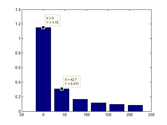
Another thing worth mentioning. In the spectral representation, the signal is calculated not at the frequency at which the algorithm hit (as we remember, the frequencies follow with the Fd / FftL step), but the value in the band (the width is equal to the step). Those. if several discretes fall into this band, they are added together. For example, you can reduce the number of lines as a result of the algorithm:
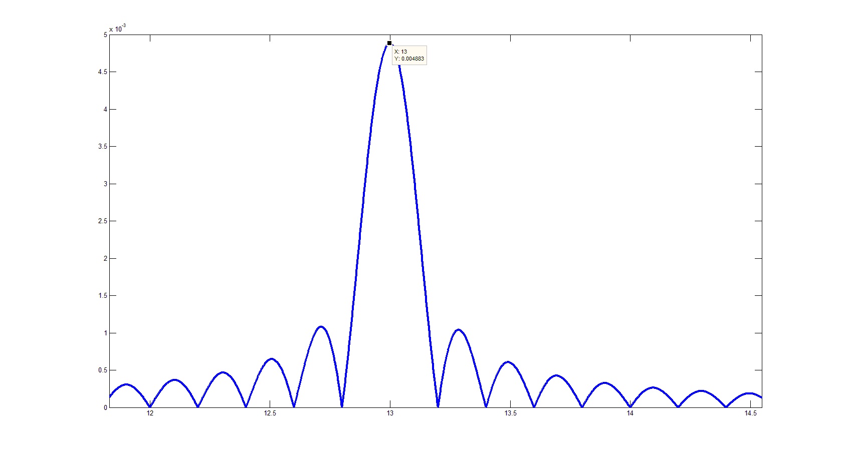
However, this does not mean that it is worthless to immediately increase the accuracy of work, since This also leads to negative consequences, because If the resolution is comparable to the sampling rate of a signal, the harmonics of the “window” will enter the spectrum, which are related not to the real signal, but to its discrete representation:
Or closer to one of the discrete neighborhoods:
The code for normalizing fft will look something like this:
%%
FftS=abs(fft(Signal,FftL));%
FftS=2*FftS./FftL;%
FftS(1)=FftS(1)/2;%
FftSh=abs(fft(Signal+Noise,FftL));% +
FftSh=2*FftSh./FftL;%
FftSh(1)=FftSh(1)/2;%
We only need to display the results. The subplot function allows you to split the window into several areas to display graphs.
%%
subplot(2,1,1);%
plot(T,Signal);%
title('');%
xlabel(' ()');%
ylabel(' ()');%
subplot(2,1,2);%
plot(T,Signal+Noise);% +
title('+');%
xlabel(' ()');%
ylabel(' ()');%

F=0:Fd/FftL:Fd/2-1/FftL;%
figure%
subplot(2,1,1);%
plot(F,FftS(1:length(F)));%
title(' ');%
xlabel(' ()');%
ylabel(' ()');%
subplot(2,1,2);%
plot(F,FftSh(1:length(F)));%
title(' ');%
xlabel(' ()');%
ylabel(' ()');%
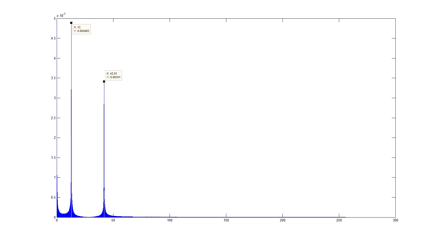
The result of the code will be as follows:
Despite the fact that the useful signal is not visible against the background of noise, the spectral characteristic allows us to determine its frequency and amplitude.
I hope this text was useful to you.
Source: https://habr.com/ru/post/112068/
All Articles