Genetic Algorithms in MATLAB

The essence of genetic algorithms

This topic is devoted to solving optimization problems using genetic algorithms in the MATLAB environment. I apologize in advance for the large amount of data: it is due to the fact that when writing a topic the main task was to disclose in detail each of the parameters of genetic algorithms that are configurable in MATLAB.

Genetic algorithms are a method for solving optimization problems based on the biological principles of natural selection and evolution. The genetic algorithm repeats a certain number of times the procedure for modifying a population (a set of individual solutions), thereby obtaining new sets of solutions (new populations). At the same time, at each step, “parents” are selected from the population, that is, solutions, the joint modification of which (crossing) leads to the formation of a new individual in the next generation. The genetic algorithm uses three types of rules on the basis of which a new generation is formed: selection, crossing and mutation rules. Mutation allows, by making changes in a new generation, to avoid falling into local minima of an optimized function.

(Under the cut the main part + a few screenshots).

')
The mechanism of working with genetic algorithms in MATLAB is implemented in two ways:

1. The call function of genetic algorithms
2. Using the Genetic Algorithm Tool Kit

Both methods are supplied in the standard set of functions and MATLAB modules. In my opinion, the second way of working with genetic algorithms in MATLAB, associated with the use of the Genetic Algorithm Tool module, is much more convenient and visual. And consider it in more detail.

Work with GENETIC ALGORITHM TOOL

To run the Genetic Algorithm Tool package, the gatool command should be executed on the MATLAB command line. After that, the genetic algorithms package will start and the main utility window will appear on the screen.



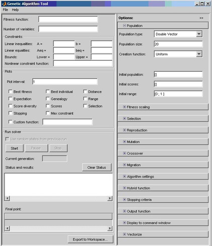
The Fitness function field indicates the function to be optimized in the form of @fitnessfun, where fitnessfun.m is the name of the M-file, in which the function to be optimized should first be described. Just in case, I note that the M-file is created in the MATLAB environment through the menu File-> New-> M-File. An example of the description of some function my_fun in the M-file:

function z = my_fun (x)
z = x (1) ^ 2 - 2 * x (1) * x (2) + 6 * x (1) + x (2) ^ 2 - 6 * x (2);

Let's return to the main GATool utility window. The Number of variables field indicates the length of the input vector of the function being optimized. In the example above, the function my_fun has an input vector of length 2.
In the Constraints panel, you can set constraints or a limiting non-linear function. In the Linear inequalities field, a linear restriction is specified by an inequality of the form:

A * x ≤ b.

In the Linear equalities field of this panel, linear restrictions are set by the equality:

A * x = b.

In both cases, A is some matrix, b is a vector.

In the Bounds field in the vector form, the lower and upper constraints of variables are specified, and in the Nonlinear constraint function field, you can specify an arbitrary nonlinear constraint function.

If the task does not require setting constraints, all fields of the Constraints panel should be left blank.

Below is the chart settings panel. It allows you to display various graphs that display information about the operation of the genetic algorithm. Based on this information, you can change the settings of the algorithm in order to increase its efficiency. For example, choosing the Best Fitness option in this panel allows you to display on one chart the best and average values ​​of the function being optimized for each generation of the algorithm. This panel will be described in more detail below along with the rest of the panels on the Options tab of the GATool utility.

The Run Solver panel contains controls (the Start, Pause and Stop buttons to start, temporarily and completely stop the genetic algorithm). It also contains the Status and results field, which displays the current results of the running genetic algorithm, and Final point, which displays the value of the end point of the algorithm - the best value of the optimized function (that is, the desired value).

On the right side of the main GATool utility window is the Options panel. It allows you to set various settings for the operation of genetic algorithms. When you click the [+] buttons, which are opposite the name of each of the adjustable parameters in the Options panel, drop-down lists (tabs) appear, containing fields for entering and changing the corresponding parameters of the genetic algorithm.



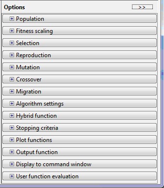
The main customizable parameters in GATool are:
- population (Population tab);
- scaling (tab Fitness Scaling);
- selection operator (Selection tab);
- Reproduction operator (Reproduction tab);
- mutation operator (Mutation tab);
- crossover operator (Crossover tab);
- transfer of individuals between populations (tab Migration);
- special algorithm parameters (Algorithm settings tab);
- setting the hybrid function (tab Hybrid function);
- setting the stopping criteria of the algorithm (Stopping criteria tab);
- output of various additional information in the course of the genetic algorithm (Plot Functions tab);
- output the results of the algorithm in the form of a new function (tab Output function);
- the task of a set of information for an output in a command window (the Display to command window tab);
- method of calculating the values ​​of the optimized and limiting functions (tab User function evaluation).

Let's take a closer look at all the above tabs of the Options panel and the elements they contain.

In the settings tab of populations, the user has the opportunity to select the type of mathematical objects to which the individuals of all populations will belong (double vector, bit string, or user-defined type). It should be borne in mind that the use of the bit string and user-defined types impose restrictions on the list of valid creation, mutation and crossing operators of individuals. Thus, for example, when selecting the bit-line as the representation form for a crossing operator, it is impossible to use a hybrid function or a non-linear constraint function.
Also, the population tab allows you to adjust the population size (of how many individuals each generation will consist of) and how the initial generation will be created (Uniform - if there are no imposed restrictions, otherwise - Feasible population). In addition, in the tab under consideration, it is possible to manually set the initial generation (using the Initial population item or its part, the initial rating of individuals (the Initial scores item), and also enter a restrictive numerical range to which the initial population individuals should belong.

In the Fitness Scaling tab, the user can specify a scaling function that converts the values ​​achieved by the function to be optimized into values ​​within the limits allowed by the selection operator. When selecting the Rank parameter as the scaling function, the scaling will be brought to the rating, that is, individuals will be assigned a rating number (one for the best individual, one for the next two, and so on). Proportional scaling sets the probabilities proportional to a given number for individuals. When selecting the Top option, the highest rating value is assigned to several of the most prominent individuals at once (their number is indicated as a parameter). Finally, when choosing the Shift linear scaling type, it is possible to specify the maximum probability of the best individual.

The Selection tab allows you to select a parent selection operator based on data from the scaling function. The following options are available for selection of operator options:

- Tournament - a specified number of individuals are randomly selected, among them the best are selected on a competitive basis;
- Roulette — simulates a roulette, in which the size of each segment is set according to its probability;
- Uniform - parents are selected randomly according to a given distribution and taking into account the number of parents and their probabilities;
- Stochastic uniform - a line is built in which each parent is assigned its part of a certain size (depending on the probability of the parent), then the algorithm runs through the sweat line in steps of the same length and selects the parents depending on which part of the line the step falls on.

The Reproduction tab clarifies how new individuals are created. The item Elite count allows you to specify the number of individuals that are guaranteed to be transferred to the next generation. Crossover fraction indicates the proportion of individuals that are created by crossing. The remaining fraction is created by mutation.

In the mutation operator tab, select the type of mutation operator. The following options are available:

- Gaussian - adds a small random number (according to the Gaussian distribution) to all components of each individual vector;
- Uniform — the components of the vectors are selected randomly and random numbers from the allowed range are written instead;
- Adaptive feasible - generates a set of directions depending on the last most successful and unsuccessful generations and, taking into account the restrictions imposed, moves along all directions to different lengths;
- Custom - allows you to set your own function.

The Crossover tab allows you to choose the type of crossover operator (single-point, two-point, heuristic, arithmetic, or scattered, which generates a random binary parent matching vector). It is also possible to set an arbitrary (custom) crossover function.

In the Migration tab, you can configure the rules according to which individuals will move between subpopulations within the same population. Subpopulations are created if a vector is specified as the size of a population, and not a natural value. In this tab, you can specify the direction of migration (forward - to the next subpopulation, both - to the previous and next), the proportion of migrating individuals and the frequency of migration (how many generations pass between migrations). If the creation of subpopulations is not required, this tab should always be left unchanged.

The special options tab of the algorithm allows you to customize the solution parameters for the system of nonlinear constraints imposed on the algorithm. The value of the Initial penalty parameter determines the initial numerical value of the critique of the algorithm, the Penalty factor is used as a multiplier of this value in cases where the developer is not satisfied with the optimization accuracy or when going beyond the boundaries defined in the restrictions tab. As a rule, these options are configured in detail for solving problems of high complexity.

The Hybrid function tab allows you to specify another minimization function, which will be used after the end of the algorithm. The following functions built into the MATLAB environment are available as possible hybrid functions:
- none (do not use the hybrid function);
- fminsearch (search for the minimum of values);
- patternsearch (search by pattern);
- fminunc (for an unlimited algorithm);
- fmincon (for an algorithm with specified constraints).

The Stopping criteria tab indicates the situations in which the algorithm makes a stop. In this case, the following parameters are customizable:

- Generations - the maximum number of generations, after which exceeding will stop;
- Time limit - time limit for the operation of the algorithm;
- Fitness limit - if the optimized value is less than or equal to the given limit, the algorithm will stop;
- Stall generations - the number of slightly different generations, after which the algorithm will stop;
- Stall time limit - the same as the previous parameter, but applicable to the running time of the algorithm;
- Function tolerance and Nonlinear constraint tolerance - the minimum values ​​of the changes of the optimized and limiting functions, respectively, at which the algorithm will continue to work.

Of particular interest is the Plot Functions tab, which allows you to select various information that is displayed in the course of the algorithm and shows both the correctness of its work and the specific results achieved by the algorithm. The most important and used parameters for display are:

- Plot interval - the number of generations, after which the next update of the graphs occurs;
- Best fitness - output the best value of the optimized function for each generation;
- Best individual - the conclusion of the best representative of the generation with the best optimization result in each of the generations;
- Distance - output the interval between the values ​​of individuals in a generation;
- Expectation - displays a number of probabilities and the corresponding individuals of generations;
- Genealogy - conclusion of the genealogical tree of individuals;
- Range — output the smallest, largest, and average values ​​of the function being optimized for each generation;
- Score diversity - display a histagram of the rating in each generation;
- Scores - displaying the rating of each individual in a generation;
- Selection - display the histogram of parents;
- Stopping - display information about the status of all parameters that affect the criteria for stopping;
- Custom - display on the graph of some user-defined function.

The output tab of the results in the form of a new function (Output function) allows you to enable the output of the history of the algorithm in a separate window with a specified generation interval (the History to new window flag and the Interval field, respectively), and also allows you to specify and output an arbitrary output function specified in the Custom field function.

The User function evaluation tab describes the order in which the values ​​of the optimized and limiting functions are calculated (separately, in parallel in one call, or simultaneously).

Finally, the Display to command window tab allows you to customize the information that is displayed in the main MATLAB command window when the algorithm is running. The following values ​​are possible: Off - no output in the command window, Iterative - output information about each iteration of the working algorithm, Diagnose - output information about each iteration and additional information about possible errors and modified key parameters of the algorithm, Final - only the reason for the stop and the final value are displayed .

PS When writing this topic, the author enjoyed the personal experience and help of the MATLAB environment. In future articles I will try to reveal the gatool mechanism described above with specific examples, both classical (optimization of the linear function, shooting tasks and traveling salesman), and some specific ones.

PPS Thank you for your attention to those who read to the end.