Heuristic investment portfolio generation algorithms
Suppose that we have $ 100 million that needs to be invested in several possible investments. Each of these investments has a different value and a different expected return. We have to decide how to spend the money in order to get the maximum profit.
Tasks of this type are called portfolio formation tasks. We have several positions (investments) that should fit in a fixed-size portfolio ($ 100 million). Each position has its own profitability. It is necessary to find a set of positions that fit into the portfolio and give the maximum profit.
Many of you will say that no heuristics are not needed here, and that it is quite possible to do a complete brute force. Others will declare that a complete search is not needed, because there is a method of branches and borders. But what if the number of possible investments is 65? A complete decision tree contains more than 7 * 10 ^ 19 nodes. Suppose that the branch and bound method goes through a tenth of a percent of these nodes, and the computer checks a million nodes per second. Under these conditions, it would take more than 2 million years to solve the problem. Heuristics are used precisely for such complex tasks. If you're interested, you are welcome under the cat.
The heuristic method of climbing a hill makes changes to the current decision, promoting it as close as possible to the goal. This process is called climbing a hill because it is similar to how a lost traveler tries to get to the top of a mountain at night. Even if it is already too dark to see something away, he can try to reach the top of the mountain, constantly moving up.
Of course, there is a possibility that the traveler will stop at the top of a smaller hill and will not reach the peak. This problem exists when using this heuristic method. The algorithm may find a solution that will be locally optimal, but will not be the best possible solution.
In the task of forming a portfolio of investments, the goal is to select a set of positions with a total value of no more than the allowable limit, and the total profit should be as large as possible. The heuristics of climbing the hill for this task chooses the position that gives the maximum profit at each step. In this case, the decision will be better to meet the goal - to maximize profits.
The algorithm first adds the position with the maximum profit to the solution, then the next position with the maximum profit is added (provided that the full price remains within acceptable limits). Joining positions with maximum profit will continue until the value limit is exhausted.
For the list of investments below, the program will first select deal A, because it has the largest profit ($ 9 million). Then C is selected because it has the largest profit out of those remaining ($ 8 million). At this point in time, of the permissible 100 million, 93 million have already been spent, and the algorithm will no longer be able to select any transactions. The solution, calculated using this heuristic, includes elements A and C, costs 93 million and yields a profit of 17 million.
Hill climbing heuristics fills the portfolio very quickly. If the elements are initially ordered in order of decreasing profits, then the complexity of the algorithm is of the order of O (N). The program simply moves through the list, adding positions with the maximum profit, until the limit of funds is reached. If the list is not sorted, then the complexity of this algorithm is N * log (N). This is much better than the O (2 ^ N) steps required to complete a search through all the nodes of the tree. For 20 positions, this heuristic uses about 400 steps, the branch and bound method uses several thousand, and the total bust is more than 2 million.
A strategy that is in some sense the opposite of the hill climb method is called the least cost method. Instead of bringing the solution as close as possible to the goal at every step, you can try to reduce the cost of the solution. In the example with the formation of a portfolio of investments at each step, a position with a minimum value is added to the solution.
This strategy will place as many positions as possible in the solution. This works well if all items have approximately the same value. But if an expensive transaction makes a big profit, this strategy may miss the chance, giving not the best possible result.
For the investments above, the minimum cost strategy begins by first adding a transaction E worth 23 million to the solution. Then it selects position D worth 27 million and C worth 30 million. At this point, the algorithm has already spent 80 million out of 100 million dollars and can no longer make a single investment.
The resulting solution costs 80 million and gives a profit of 18 million. This is a million better than a solution that a heuristic of climbing a hill gives us, but the minimum cost algorithm does not always work more efficiently than a hill climbing algorithm. Which method will give the best solution depends on the specific data.
The structure of programs that implement heuristics of minimum cost and hill climbing heuristics is almost identical. The only difference is in choosing the next position, which is added to the existing solution. The minimum cost method instead of the position with the maximum profit selects the position that has the lowest cost. Since the two methods are very similar, their complexity is the same. If the positions are properly sorted, both algorithms have complexity of the order of O (N). With a random arrangement of positions, their complexity will be of the order of O (N * log (N)).
Hill climbing strategy does not take into account the value of the added positions. She chooses positions with maximum profit, even if they have a greater value. The minimum value strategy does not take into account the profit brought by the position. She chooses items at a low cost, even if they have a small profit.
The heuristic of the balanced profit compares both the profit and the value of the positions to determine which positions to select. At each step, the heuristics selects the element with the largest ratio of profit to value (provided that after the investment is included in the portfolio, the total price remains within acceptable limits).
We include a new column in the table - the profit / cost ratio. With this approach, the position C is chosen first, because it has the highest ratio - 0.27. Then D is added with a ratio of 0.26 and B with a ratio of 0.20. At this point, 92 million out of 100 million has been spent, and no position can be added to the solution.
This solution has a cost of 92 million and yields a profit of 22 million. This is 4 million better than the solution found using the minimum cost method and 5 million better than the solution found by heuristics of climbing a hill. Moreover, the solution found will generally be the best of all possible, which will be confirmed by a search by a full search or the branch and bound method. But it is important to understand that a balanced profit is still a heuristic, therefore with the help of this it is not always possible to find the best possible solution. Very often, this method finds better solutions than solutions found using hill climbing methods and minimal cost, but this does not always happen. The structure of the program that implements the heuristic of balanced profit is almost identical to the structure of the hill climbing program and the minimum cost. The only difference is in the method of choosing the next position that is added to the solution. The complexity of this heuristic is proportional to O (N), subject to pre-sorting. If the positions are arranged arbitrarily, the complexity of the algorithm will be O (N * log (N)).
Random search is performed according to its name. At each step, the algorithm adds a randomly selected position that satisfies the cost limits. This type of enumeration is called the Monte Carlo method.
Since a randomly chosen solution is unlikely to be the best, in order to obtain an acceptable result, it is necessary to repeat the search several times. Although at first glance it seems that the probability of finding a good solution is very small, the use of this method sometimes brings surprisingly good results. Depending on the source data and the number of checked random solutions, this heuristic often works better than hill climb methods and minimal cost.
The advantage of random searching is that this method is easy to understand and implement. It is sometimes difficult to imagine how to implement a hill climbing method, minimum cost, or reduced profit, but it is always easy to generate solutions at random. Even to solve extremely complex problems, random search is the easiest method.
Another strategy is to start with a random decision and then make a sequential approximation. Starting with a randomly generated solution, the program makes a random selection. If the new solution is an improvement of the previous one, the program fixes the change and continues checking other positions. If the change does not improve the solution, the program abandons it and makes a new attempt.
It is especially easy to implement a method of sequential approximation for the problem of forming a portfolio of investments. The program only chooses a random position from the trial solution and removes it from the current one. Then it randomly adds positions to the solution until the limit of funds is reached. If a remote position had a very high cost, then the program may not add several positions to its place.
Like the random search, this heuristic is easy to understand and implement. To solve a complex problem, it can be hard to create algorithms for climbing a hill, the minimum cost, and reduced profit, but it is fairly easy to write a heuristic algorithm of successive approximation.
There are several good ways to determine when to stop random changes. For example, it is allowed to make a fixed number of changes. For a task of N elements, you can perform N or N ^ 2 random changes and then stop the program execution.
Another strategy is to make changes as long as successive changes will bring improvements. As soon as a few consecutive changes do not give improvements, the program can be stopped.
If a program replaces a randomly selected position in a trial solution, it may find a solution that cannot be improved, but it still will not be the best possible solution. As an example, consider the following set of possible investments.
Suppose that the algorithm randomly selects positions A and B as the initial solution. Its value will be equal to 90 million, it will bring a profit of 17 million.
If the program removes either A or B, then the solution will have a fairly large cost, so the program will be able to add only one new position. Since positions A and B have the largest profit, replacing them with another position will reduce the total profit. Accidental deletion of one position from this solution will never lead to improvement.
The best solution contains positions C, D, E. Its full value is equal to 98 million, the total profit is 18 million. To find this solution, the algorithm must remove both positions A and B from the solution and add new ones to their place.
Such solutions, when small changes cannot improve solutions, are called local optimum. There are two ways in which the program will not stop at the local optimum, but will seek a global optimum.
First, the program can be modified so that it removes several positions from the solution. If the program deletes two randomly selected positions, it can find the right solution for this example. However, for larger tasks, removing two items is usually not enough. The program will need to remove three, four, and maybe a larger number of positions.
A simpler way is to perform a larger number of tests with different initial solutions. Some of the initial decisions can lead to local optima, but one of them will allow to achieve a global optimum.
The annealing method is borrowed from thermodynamics. During annealing, the metal is heated to a high temperature. Molecules in the hot metal make rapid vibrations. If the metal is slowly cooled, then the molecules begin to line up, forming crystals. In this case, the molecules gradually pass into a state with minimal energy.
When the metal cools, adjacent crystals merge with each other. Molecules of one crystal temporarily leave their positions with minimal energy and combine with molecules of another crystal. The energy of the resulting larger crystal will be less than the sum of the energies of the two original crystals. If the metal is cooled slowly enough, the crystals will become huge. The final arrangement of the molecules will have a very low total energy, so the metal will be very strong.
Starting from a high energy state, the molecules eventually reach a low energy state. On the way to the final position, they pass through many local energy minima. Each combination of crystals represents a local minimum. Bringing the crystal to the minimum energy state is possible only by temporal resolution of the structure of smaller crystals, thereby increasing the energy of the system, as a result of which the crystals can be combined.
The annealing method uses a similar method of finding the best solution to the problem. When a program looks for a solution, it can get stuck in a local optimum. To avoid this, it makes random changes to the decision from time to time, even if the next option does not lead to an instant result improvement. This allows the program to exit the local optimum and find the best solution.
So that the program does not get hung up on these modifications, the algorithm after some time changes the probability of introducing random changes. The probability of making one change is P = 1 / e ^ (E / (k * T)), where E is the amount of “energy” added to the system, k is a constant chosen depending on the type of task and T is a variable corresponding to “temperature ".
First, the value of T should be quite high, so the likelihood of changes will also be quite high. After some time, the value of T decreases, and the probability of random changes also decreases. Once the process has reached a point at which no changes can improve the solution and the value of T becomes so small that random changes are very rare, the algorithm will finish.
For the task of forming a portfolio of investments, E is the amount by which the profit is reduced as a result of the change. For example, if we delete a position whose profit is equal to 10 million dollars, and replace it with a position having a profit of 7 million dollars, the energy added to the system will be 3. If the value of E is large, then the probability of change is small, therefore the probability of large changes below.
Different heuristic methods behave differently in different tasks. The heuristics of a balanced profit is good enough to solve the problem of forming a portfolio of investments, given its simplicity. The strategy of successive approximation also works quite well, but it takes much longer. For other problems, some other heuristics may be best, including those not discussed in this chapter.
Heuristics work much faster than full brute force and branch and bound methods. Some heuristic approaches (hill climbing, minimum cost, balanced profit, etc.) work extremely quickly because they only consider one possible solution. These methods work so fast that sometimes it makes sense to do them all in turn, and then choose the best of the three solutions obtained. Of course, it is impossible to guarantee that this solution will be the best, but it will definitely be good enough.
Tasks of this type are called portfolio formation tasks. We have several positions (investments) that should fit in a fixed-size portfolio ($ 100 million). Each position has its own profitability. It is necessary to find a set of positions that fit into the portfolio and give the maximum profit.
Many of you will say that no heuristics are not needed here, and that it is quite possible to do a complete brute force. Others will declare that a complete search is not needed, because there is a method of branches and borders. But what if the number of possible investments is 65? A complete decision tree contains more than 7 * 10 ^ 19 nodes. Suppose that the branch and bound method goes through a tenth of a percent of these nodes, and the computer checks a million nodes per second. Under these conditions, it would take more than 2 million years to solve the problem. Heuristics are used precisely for such complex tasks. If you're interested, you are welcome under the cat.
Hill climbing
The heuristic method of climbing a hill makes changes to the current decision, promoting it as close as possible to the goal. This process is called climbing a hill because it is similar to how a lost traveler tries to get to the top of a mountain at night. Even if it is already too dark to see something away, he can try to reach the top of the mountain, constantly moving up.
Of course, there is a possibility that the traveler will stop at the top of a smaller hill and will not reach the peak. This problem exists when using this heuristic method. The algorithm may find a solution that will be locally optimal, but will not be the best possible solution.
In the task of forming a portfolio of investments, the goal is to select a set of positions with a total value of no more than the allowable limit, and the total profit should be as large as possible. The heuristics of climbing the hill for this task chooses the position that gives the maximum profit at each step. In this case, the decision will be better to meet the goal - to maximize profits.
The algorithm first adds the position with the maximum profit to the solution, then the next position with the maximum profit is added (provided that the full price remains within acceptable limits). Joining positions with maximum profit will continue until the value limit is exhausted.
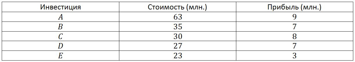
For the list of investments below, the program will first select deal A, because it has the largest profit ($ 9 million). Then C is selected because it has the largest profit out of those remaining ($ 8 million). At this point in time, of the permissible 100 million, 93 million have already been spent, and the algorithm will no longer be able to select any transactions. The solution, calculated using this heuristic, includes elements A and C, costs 93 million and yields a profit of 17 million.
Hill climbing heuristics fills the portfolio very quickly. If the elements are initially ordered in order of decreasing profits, then the complexity of the algorithm is of the order of O (N). The program simply moves through the list, adding positions with the maximum profit, until the limit of funds is reached. If the list is not sorted, then the complexity of this algorithm is N * log (N). This is much better than the O (2 ^ N) steps required to complete a search through all the nodes of the tree. For 20 positions, this heuristic uses about 400 steps, the branch and bound method uses several thousand, and the total bust is more than 2 million.
Least Cost Method
A strategy that is in some sense the opposite of the hill climb method is called the least cost method. Instead of bringing the solution as close as possible to the goal at every step, you can try to reduce the cost of the solution. In the example with the formation of a portfolio of investments at each step, a position with a minimum value is added to the solution.
This strategy will place as many positions as possible in the solution. This works well if all items have approximately the same value. But if an expensive transaction makes a big profit, this strategy may miss the chance, giving not the best possible result.
For the investments above, the minimum cost strategy begins by first adding a transaction E worth 23 million to the solution. Then it selects position D worth 27 million and C worth 30 million. At this point, the algorithm has already spent 80 million out of 100 million dollars and can no longer make a single investment.
The resulting solution costs 80 million and gives a profit of 18 million. This is a million better than a solution that a heuristic of climbing a hill gives us, but the minimum cost algorithm does not always work more efficiently than a hill climbing algorithm. Which method will give the best solution depends on the specific data.
The structure of programs that implement heuristics of minimum cost and hill climbing heuristics is almost identical. The only difference is in choosing the next position, which is added to the existing solution. The minimum cost method instead of the position with the maximum profit selects the position that has the lowest cost. Since the two methods are very similar, their complexity is the same. If the positions are properly sorted, both algorithms have complexity of the order of O (N). With a random arrangement of positions, their complexity will be of the order of O (N * log (N)).
Balanced profit
Hill climbing strategy does not take into account the value of the added positions. She chooses positions with maximum profit, even if they have a greater value. The minimum value strategy does not take into account the profit brought by the position. She chooses items at a low cost, even if they have a small profit.
The heuristic of the balanced profit compares both the profit and the value of the positions to determine which positions to select. At each step, the heuristics selects the element with the largest ratio of profit to value (provided that after the investment is included in the portfolio, the total price remains within acceptable limits).
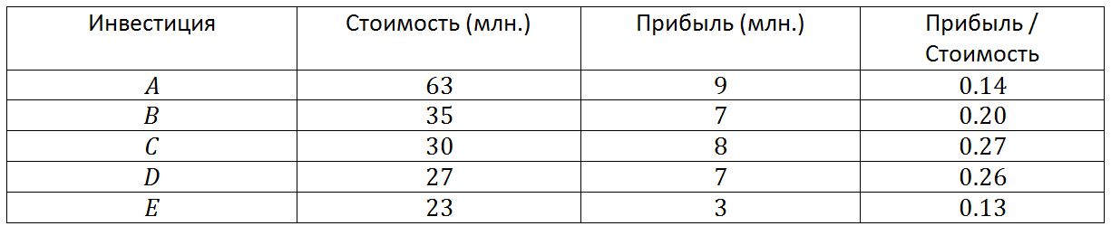
We include a new column in the table - the profit / cost ratio. With this approach, the position C is chosen first, because it has the highest ratio - 0.27. Then D is added with a ratio of 0.26 and B with a ratio of 0.20. At this point, 92 million out of 100 million has been spent, and no position can be added to the solution.
This solution has a cost of 92 million and yields a profit of 22 million. This is 4 million better than the solution found using the minimum cost method and 5 million better than the solution found by heuristics of climbing a hill. Moreover, the solution found will generally be the best of all possible, which will be confirmed by a search by a full search or the branch and bound method. But it is important to understand that a balanced profit is still a heuristic, therefore with the help of this it is not always possible to find the best possible solution. Very often, this method finds better solutions than solutions found using hill climbing methods and minimal cost, but this does not always happen. The structure of the program that implements the heuristic of balanced profit is almost identical to the structure of the hill climbing program and the minimum cost. The only difference is in the method of choosing the next position that is added to the solution. The complexity of this heuristic is proportional to O (N), subject to pre-sorting. If the positions are arranged arbitrarily, the complexity of the algorithm will be O (N * log (N)).
Random methods
Random search
Random search is performed according to its name. At each step, the algorithm adds a randomly selected position that satisfies the cost limits. This type of enumeration is called the Monte Carlo method.
Since a randomly chosen solution is unlikely to be the best, in order to obtain an acceptable result, it is necessary to repeat the search several times. Although at first glance it seems that the probability of finding a good solution is very small, the use of this method sometimes brings surprisingly good results. Depending on the source data and the number of checked random solutions, this heuristic often works better than hill climb methods and minimal cost.
The advantage of random searching is that this method is easy to understand and implement. It is sometimes difficult to imagine how to implement a hill climbing method, minimum cost, or reduced profit, but it is always easy to generate solutions at random. Even to solve extremely complex problems, random search is the easiest method.
Sequential approximation
Another strategy is to start with a random decision and then make a sequential approximation. Starting with a randomly generated solution, the program makes a random selection. If the new solution is an improvement of the previous one, the program fixes the change and continues checking other positions. If the change does not improve the solution, the program abandons it and makes a new attempt.
It is especially easy to implement a method of sequential approximation for the problem of forming a portfolio of investments. The program only chooses a random position from the trial solution and removes it from the current one. Then it randomly adds positions to the solution until the limit of funds is reached. If a remote position had a very high cost, then the program may not add several positions to its place.
Like the random search, this heuristic is easy to understand and implement. To solve a complex problem, it can be hard to create algorithms for climbing a hill, the minimum cost, and reduced profit, but it is fairly easy to write a heuristic algorithm of successive approximation.
Moment of stopping
There are several good ways to determine when to stop random changes. For example, it is allowed to make a fixed number of changes. For a task of N elements, you can perform N or N ^ 2 random changes and then stop the program execution.
Another strategy is to make changes as long as successive changes will bring improvements. As soon as a few consecutive changes do not give improvements, the program can be stopped.
Local optimum
If a program replaces a randomly selected position in a trial solution, it may find a solution that cannot be improved, but it still will not be the best possible solution. As an example, consider the following set of possible investments.
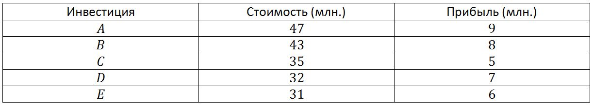
Suppose that the algorithm randomly selects positions A and B as the initial solution. Its value will be equal to 90 million, it will bring a profit of 17 million.
If the program removes either A or B, then the solution will have a fairly large cost, so the program will be able to add only one new position. Since positions A and B have the largest profit, replacing them with another position will reduce the total profit. Accidental deletion of one position from this solution will never lead to improvement.
The best solution contains positions C, D, E. Its full value is equal to 98 million, the total profit is 18 million. To find this solution, the algorithm must remove both positions A and B from the solution and add new ones to their place.
Such solutions, when small changes cannot improve solutions, are called local optimum. There are two ways in which the program will not stop at the local optimum, but will seek a global optimum.
First, the program can be modified so that it removes several positions from the solution. If the program deletes two randomly selected positions, it can find the right solution for this example. However, for larger tasks, removing two items is usually not enough. The program will need to remove three, four, and maybe a larger number of positions.
A simpler way is to perform a larger number of tests with different initial solutions. Some of the initial decisions can lead to local optima, but one of them will allow to achieve a global optimum.
Annealing method
The annealing method is borrowed from thermodynamics. During annealing, the metal is heated to a high temperature. Molecules in the hot metal make rapid vibrations. If the metal is slowly cooled, then the molecules begin to line up, forming crystals. In this case, the molecules gradually pass into a state with minimal energy.
When the metal cools, adjacent crystals merge with each other. Molecules of one crystal temporarily leave their positions with minimal energy and combine with molecules of another crystal. The energy of the resulting larger crystal will be less than the sum of the energies of the two original crystals. If the metal is cooled slowly enough, the crystals will become huge. The final arrangement of the molecules will have a very low total energy, so the metal will be very strong.
Starting from a high energy state, the molecules eventually reach a low energy state. On the way to the final position, they pass through many local energy minima. Each combination of crystals represents a local minimum. Bringing the crystal to the minimum energy state is possible only by temporal resolution of the structure of smaller crystals, thereby increasing the energy of the system, as a result of which the crystals can be combined.
The annealing method uses a similar method of finding the best solution to the problem. When a program looks for a solution, it can get stuck in a local optimum. To avoid this, it makes random changes to the decision from time to time, even if the next option does not lead to an instant result improvement. This allows the program to exit the local optimum and find the best solution.
So that the program does not get hung up on these modifications, the algorithm after some time changes the probability of introducing random changes. The probability of making one change is P = 1 / e ^ (E / (k * T)), where E is the amount of “energy” added to the system, k is a constant chosen depending on the type of task and T is a variable corresponding to “temperature ".
First, the value of T should be quite high, so the likelihood of changes will also be quite high. After some time, the value of T decreases, and the probability of random changes also decreases. Once the process has reached a point at which no changes can improve the solution and the value of T becomes so small that random changes are very rare, the algorithm will finish.
For the task of forming a portfolio of investments, E is the amount by which the profit is reduced as a result of the change. For example, if we delete a position whose profit is equal to 10 million dollars, and replace it with a position having a profit of 7 million dollars, the energy added to the system will be 3. If the value of E is large, then the probability of change is small, therefore the probability of large changes below.
Comparing Heuristic Methods
Different heuristic methods behave differently in different tasks. The heuristics of a balanced profit is good enough to solve the problem of forming a portfolio of investments, given its simplicity. The strategy of successive approximation also works quite well, but it takes much longer. For other problems, some other heuristics may be best, including those not discussed in this chapter.
Heuristics work much faster than full brute force and branch and bound methods. Some heuristic approaches (hill climbing, minimum cost, balanced profit, etc.) work extremely quickly because they only consider one possible solution. These methods work so fast that sometimes it makes sense to do them all in turn, and then choose the best of the three solutions obtained. Of course, it is impossible to guarantee that this solution will be the best, but it will definitely be good enough.
')
Source: https://habr.com/ru/post/108961/
All Articles