Classification of data by the support vector machine
Good day!
In this article I want to talk about the problem of classifying data using the Support Vector Machine (SVM). This classification has a fairly wide application: from pattern recognition or the creation of spam filters to calculate the distribution of hot aluminum particles in rocket exhaust.
First, a few words about the original problem. The task of classification is to determine which class of at least two initially known objects this object belongs to. Typically, such an object is a vector in n- dimensional real space . The coordinates of the vector describe the individual attributes of the object. For example, the color c specified in the RGB model is a vector in three-dimensional space: c = ( red, green, blue ).
')
If there are only two classes (“spam / not spam”, “give credit / not give credit”, “red / black”), then the problem is called binary classification. If there are several classes, a multi-class (multi-class) classification. There may also be samples of each class - objects about which it is known in advance to which class they belong. Such tasks are called learning with a teacher , and known data is called a learning sample . (Note: if classes are not initially set, then we have a clustering task. )
The support vector method discussed in this article is about learning with a teacher.
So, the mathematical formulation of the classification problem is as follows: let X be an object space (for example, ), Y - our classes (for example, Y = {-1,1}). Dana training sample:  . Required to build a function
  (classifier) associating the class y with an arbitrary object x.
This method initially refers to binary classifiers, although there are ways to make it work for multiclassification tasks.
It is convenient to illustrate the idea of the method in the following simple example: the points in the plane are divided into two classes (Fig. 1). Let's draw a line separating these two classes (the red line in Fig. 1). Further, all new points (not from the training set) are automatically classified as follows:
the point above the line falls into class A ,
the point below the line is in class B.
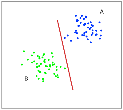
Such a line is called the dividing line. However, in spaces of high dimensions, the straight will no longer divide our classes, since the concept of “below the line” or “above the line” loses all meaning. Therefore, instead of straight lines, it is necessary to consider hyperplanes — spaces whose dimension is one less than the dimension of the original space. AT For example, a hyperplane is a regular two-dimensional plane.
In our example, there are several straight lines separating two classes (Fig. 2):

From the point of view of classification accuracy, it is best to choose a straight line, the distance from which to each class is maximum. In other words, we choose the straight line that separates the classes in the best way (the red straight line in Fig. 2). Such a straight line, and in the general case a hyperplane, is called the optimal separating hyperplane.
The vectors that are closest to the separating hyperplane are called support vectors. In Figure 2, they are marked in red.
Let there is a training set: .
.
The support vector machine builds the classification function F in the form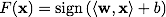 ,
,
Where Is the scalar product, w is a normal vector to the dividing hyperplane, b is an auxiliary parameter. Those objects for which F ( x ) = 1 fall into one class, and objects with F ( x ) = -1 into another. The choice of such a function is not accidental: any hyperplane can be given in the form
  for some w and b.
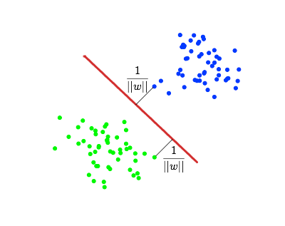
Next, we want to choose such w and b which maximize the distance to each class. It can be calculated that this distance is equal to . The problem of finding the maximum equivalent to the problem of finding a minimum
  . We write it all in the form of an optimization problem:

which is a standard quadratic programming problem and is solved using Lagrange multipliers. A description of this method can be found on Wikipedia.
In practice, cases where the data can be divided by a hyperplane, or, as they say, linear , are quite rare. An example of linear inseparability can be seen in Figure 3:

In this case, do this: all the elements of the training sample are embedded in the space X of a higher dimension using a special mapping . With this mapping
  is chosen so that in the new space X the sample is linearly separable.
The classifying function F takes the form . Expression
  called the classifier kernel . From a mathematical point of view, the core can be any positive definite symmetric function of two variables. Positive definiteness is necessary for the corresponding Lagrange function in the optimization problem to be bounded below, i.e. optimization task would be correctly defined.
The accuracy of the classifier depends, in particular, on the choice of the core. In the video, you can see an illustration of classification using a polynomial kernel:
The most common in practice are the following cores:
Polynomial:
Radial basic function:
Gaussian radial basis function:
Sigmoid:
Among other classifiers I want to mention also the method of relevant vectors (Relevance Vector Machine, RVM). Unlike SVM, this method gives the probabilities with which an object belongs to a given class. Those. if the SVM says " x belongs to class A", then the RVM says " x belongs to class A with probability p and class B with probability 1-p ".
1. Christopher M. Bishop. Pattern recognition and machine learning, 2006.
2. K.V. Vorontsov. Lectures on the support vectors method.
In this article I want to talk about the problem of classifying data using the Support Vector Machine (SVM). This classification has a fairly wide application: from pattern recognition or the creation of spam filters to calculate the distribution of hot aluminum particles in rocket exhaust.
First, a few words about the original problem. The task of classification is to determine which class of at least two initially known objects this object belongs to. Typically, such an object is a vector in n- dimensional real space
. The coordinates of the vector describe the individual attributes of the object. For example, the color c specified in the RGB model is a vector in three-dimensional space: c = ( red, green, blue ).')
If there are only two classes (“spam / not spam”, “give credit / not give credit”, “red / black”), then the problem is called binary classification. If there are several classes, a multi-class (multi-class) classification. There may also be samples of each class - objects about which it is known in advance to which class they belong. Such tasks are called learning with a teacher , and known data is called a learning sample . (Note: if classes are not initially set, then we have a clustering task. )
The support vector method discussed in this article is about learning with a teacher.
So, the mathematical formulation of the classification problem is as follows: let X be an object space (for example,
), Y - our classes (for example, Y = {-1,1}). Dana training sample: . Required to build a function (classifier) associating the class y with an arbitrary object x.Support Vector Machine
This method initially refers to binary classifiers, although there are ways to make it work for multiclassification tasks.
Idea of the method
It is convenient to illustrate the idea of the method in the following simple example: the points in the plane are divided into two classes (Fig. 1). Let's draw a line separating these two classes (the red line in Fig. 1). Further, all new points (not from the training set) are automatically classified as follows:
the point above the line falls into class A ,
the point below the line is in class B.
Such a line is called the dividing line. However, in spaces of high dimensions, the straight will no longer divide our classes, since the concept of “below the line” or “above the line” loses all meaning. Therefore, instead of straight lines, it is necessary to consider hyperplanes — spaces whose dimension is one less than the dimension of the original space. AT
For example, a hyperplane is a regular two-dimensional plane.In our example, there are several straight lines separating two classes (Fig. 2):
From the point of view of classification accuracy, it is best to choose a straight line, the distance from which to each class is maximum. In other words, we choose the straight line that separates the classes in the best way (the red straight line in Fig. 2). Such a straight line, and in the general case a hyperplane, is called the optimal separating hyperplane.
The vectors that are closest to the separating hyperplane are called support vectors. In Figure 2, they are marked in red.
A bit of math
Let there is a training set:
.The support vector machine builds the classification function F in the form
,Where
Is the scalar product, w is a normal vector to the dividing hyperplane, b is an auxiliary parameter. Those objects for which F ( x ) = 1 fall into one class, and objects with F ( x ) = -1 into another. The choice of such a function is not accidental: any hyperplane can be given in the form for some w and b.Next, we want to choose such w and b which maximize the distance to each class. It can be calculated that this distance is equal to
. The problem of finding the maximum equivalent to the problem of finding a minimum . We write it all in the form of an optimization problem:which is a standard quadratic programming problem and is solved using Lagrange multipliers. A description of this method can be found on Wikipedia.
Linear inseparability
In practice, cases where the data can be divided by a hyperplane, or, as they say, linear , are quite rare. An example of linear inseparability can be seen in Figure 3:
In this case, do this: all the elements of the training sample are embedded in the space X of a higher dimension using a special mapping
. With this mapping is chosen so that in the new space X the sample is linearly separable.The classifying function F takes the form
. Expression called the classifier kernel . From a mathematical point of view, the core can be any positive definite symmetric function of two variables. Positive definiteness is necessary for the corresponding Lagrange function in the optimization problem to be bounded below, i.e. optimization task would be correctly defined.The accuracy of the classifier depends, in particular, on the choice of the core. In the video, you can see an illustration of classification using a polynomial kernel:
The most common in practice are the following cores:
Polynomial:
Radial basic function:
Gaussian radial basis function:
Sigmoid:
Conclusion and literature
Among other classifiers I want to mention also the method of relevant vectors (Relevance Vector Machine, RVM). Unlike SVM, this method gives the probabilities with which an object belongs to a given class. Those. if the SVM says " x belongs to class A", then the RVM says " x belongs to class A with probability p and class B with probability 1-p ".
1. Christopher M. Bishop. Pattern recognition and machine learning, 2006.
2. K.V. Vorontsov. Lectures on the support vectors method.
Source: https://habr.com/ru/post/105220/
All Articles