Evaluation of the complexity of the algorithms
Not long ago, I was offered a course of fundamentals of the theory of algorithms in one Moscow lyceum. I, of course, gladly agreed. On Monday there was the first lecture in which I tried to explain to the children methods of estimating the complexity of algorithms. I think that to some readers of Habr this information may also be useful, or at least interesting.
There are several ways to measure the complexity of an algorithm. Programmers usually focus on the speed of the algorithm, but other indicators are no less important - requirements for the amount of memory, free disk space. Using a fast algorithm will not produce the expected results if it takes more memory than its computer will need for its operation.
Many algorithms offer a choice between memory and speed. The problem can be solved quickly, using a large amount of memory, or more slowly, taking up less space.
A typical example in this case is the shortest path search algorithm. By presenting a city map as a network, you can write an algorithm to determine the shortest distance between any two points of this network. In order not to calculate these distances whenever we need them, we can derive the shortest distances between all points and save the results in a table. When we need to know the shortest distance between two given points, we can simply take the finished distance from the table.
The result will be obtained instantly, but it will require a huge amount of memory. A large city map can contain tens of thousands of points. Then, the table described above should contain more than 10 billion cells. Those. in order to improve the performance of the algorithm, you must use an additional 10 GB of memory.
The idea of volume-time complexity arises from this dependence. With this approach, the algorithm is estimated, both from the point of view of execution speed, and from the point of view of consumed memory.
We will focus on the time complexity, but, nevertheless, we will certainly stipulate the amount of memory consumed.
When comparing different algorithms, it is important to know how their complexity depends on the amount of input data. For example, when sorting with one method, processing thousands of numbers takes 1 second, and processing a million numbers takes 10 seconds. Using another algorithm, it may take 2 seconds. and 5 s. respectively. In such conditions, it is impossible to say unequivocally which algorithm is better.
In general, the complexity of the algorithm can be estimated in order of magnitude. The algorithm has complexity O (f (n)), if with increasing the dimension of the input data N, the execution time of the algorithm increases with the same speed as the function f (N). Consider the code that, for the matrix A [NxN], finds the maximum element in each row.
In this algorithm, the variable i changes from 1 to N. With each change of i, the variable j also changes from 1 to N. During each of the N iterations of the outer loop, the inner loop is also executed N times. The total number of iterations of the inner loop is N * N. This determines the complexity of the algorithm O (N ^ 2).
Evaluating the order of complexity of the algorithm, it is necessary to use only the part that increases the fastest. Suppose that the work cycle is described by the expression N ^ 3 + N. In this case, its complexity will be equal to O (N ^ 3). Consideration of the rapidly growing part of the function allows us to estimate the behavior of the algorithm with increasing N. For example, for N = 100, the difference between N ^ 3 + N = 1000100 and N = 1000000 is only 100, which is 0.01%.
When calculating O, you can ignore the constant factors in the expressions. The algorithm with a working step of 3N ^ 3 is considered as O (N ^ 3). This makes the dependence of the O (N) ratio on resizing a task more obvious.
The most difficult parts of a program are usually looping and calling procedures. In the previous example, the entire algorithm was performed using two cycles.
If one procedure causes another, it is necessary to more thoroughly assess the complexity of the latter. If a certain number of instructions are executed in it (for example, printing), this hardly affects the estimate of complexity. If, in the called procedure, O (N) steps are performed, then the function can significantly complicate the algorithm. If the procedure is called inside the loop, then the effect can be much greater.
As an example, consider two procedures: Slow with complexity O (N ^ 3) and Fast with complexity O (N ^ 2).
If the internal cycles of the Fast procedure call the Slow procedure, then the complexity of the procedures are multiplied. In this case, the complexity of the algorithm is O (N ^ 2) * O (N ^ 3) = O (N ^ 5).
If the main program calls the procedures in turn, then their complexity is added: O (N ^ 2) + O (N ^ 3) = O (N ^ 3). The following snippet has exactly this complexity:
Recall that recursive procedures are procedures that call themselves. Their complexity is quite difficult to determine. The complexity of these algorithms depends not only on the complexity of internal loops, but also on the number of iterations of recursion. A recursive procedure can look quite simple, but it can seriously complicate a program by repeatedly calling itself.
Consider a recursive implementation of factorial computation:
This procedure is performed N times, so the computational complexity of this algorithm is O (N).
A recursive algorithm that calls itself several times is called multiple recursion. Such procedures are much more difficult to analyze, in addition, they can make the algorithm much more difficult.
Consider this procedure:
Since the procedure is called twice, one would assume that its working cycle would be O (2N) = O (N). But in fact, the situation is much more complicated. If you carefully examine this algorithm, it becomes obvious that its complexity is O (2 ^ (N + 1) -1) = O (2 ^ N). You should always remember that the analysis of the complexity of recursive algorithms is a very nontrivial task.
For all recursive algorithms, the concept of bulk complexity is very important. With each call, the procedure requests a small amount of memory, but this amount may increase significantly during recursive calls. For this reason, it is always necessary to carry out at least a superficial analysis of the bulk complexity of recursive procedures.
An estimate of the complexity of the algorithm to order is the upper limit of the complexity of the algorithms. If the program has a large order of complexity, this does not mean that the algorithm will run for really long. On some data sets, the execution of the algorithm takes much less time than can be assumed based on their complexity. For example, consider the code that searches for a given element in vector A.
If the desired item is at the end of the list, then the program will have to perform N steps. In this case, the complexity of the algorithm will be O (N). In this worst case, the running time of the algorithm will be maximum.
On the other hand, the desired item may be in the list in the first position. The algorithm will have to take just one step. Such a case is called the best and its complexity can be estimated as O (1).
Both of these cases are unlikely. We are most interested in the expected option. If a list item is initially randomly mixed, then the item you are looking for may be anywhere in the list. On average, you will need to do N / 2 comparisons to find the desired item. So the complexity of this algorithm is on average O (N / 2) = O (N).
In this case, the average and expected complexity are the same, but for many algorithms the worst case is very different from the expected one. For example, in the worst case, the fast sorting algorithm has a complexity of the order of O (N ^ 2), while the expected behavior is described by the O (N * log (N)) estimate, which is much faster.
We will now list some of the functions that are most often used to calculate complexity. Functions are listed in order of increasing complexity. The higher the function in this list, the faster the algorithm will be executed with such an estimate.
1. C - constant
2. log (log (N))
3. log (N)
4. N ^ C, 0 <C <1
5. N
6. N * log (N)
7. N ^ C, C> 1
8. C ^ N, C> 1
9. N!
If we want to estimate the complexity of an algorithm whose complexity equation contains several of these functions, then the equation can be reduced to a function located in the table below. For example, O (log (N) + N!) = O (N!).
If the algorithm is rarely called for small amounts of data, then O (N ^ 2) complexity can be considered acceptable; if the algorithm works in real time, then O (N) performance is not always sufficient.
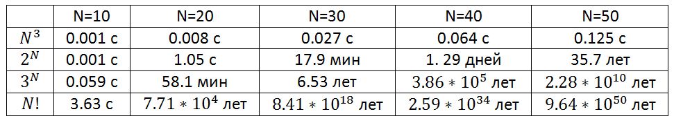
Usually algorithms with complexity N * log (N) work with good speed. Algorithms with complexity N ^ C can be used only for small values of C. The computational complexity of algorithms, the order of which is determined by the functions C ^ N and N! is very large, so these algorithms can only be used to process a small amount of data.
In conclusion, we present a table that shows how long a computer performing a million operations per second will perform some slow algorithms.
There are several ways to measure the complexity of an algorithm. Programmers usually focus on the speed of the algorithm, but other indicators are no less important - requirements for the amount of memory, free disk space. Using a fast algorithm will not produce the expected results if it takes more memory than its computer will need for its operation.
Memory or time
Many algorithms offer a choice between memory and speed. The problem can be solved quickly, using a large amount of memory, or more slowly, taking up less space.
A typical example in this case is the shortest path search algorithm. By presenting a city map as a network, you can write an algorithm to determine the shortest distance between any two points of this network. In order not to calculate these distances whenever we need them, we can derive the shortest distances between all points and save the results in a table. When we need to know the shortest distance between two given points, we can simply take the finished distance from the table.
The result will be obtained instantly, but it will require a huge amount of memory. A large city map can contain tens of thousands of points. Then, the table described above should contain more than 10 billion cells. Those. in order to improve the performance of the algorithm, you must use an additional 10 GB of memory.
The idea of volume-time complexity arises from this dependence. With this approach, the algorithm is estimated, both from the point of view of execution speed, and from the point of view of consumed memory.
We will focus on the time complexity, but, nevertheless, we will certainly stipulate the amount of memory consumed.
Order evaluation
When comparing different algorithms, it is important to know how their complexity depends on the amount of input data. For example, when sorting with one method, processing thousands of numbers takes 1 second, and processing a million numbers takes 10 seconds. Using another algorithm, it may take 2 seconds. and 5 s. respectively. In such conditions, it is impossible to say unequivocally which algorithm is better.
In general, the complexity of the algorithm can be estimated in order of magnitude. The algorithm has complexity O (f (n)), if with increasing the dimension of the input data N, the execution time of the algorithm increases with the same speed as the function f (N). Consider the code that, for the matrix A [NxN], finds the maximum element in each row.
for i:=1 to N do
begin
max:=A[i,1];
for j:=1 to N do
begin
if A[i,j]>max then
max:=A[i,j]
end;
writeln(max);
end;
In this algorithm, the variable i changes from 1 to N. With each change of i, the variable j also changes from 1 to N. During each of the N iterations of the outer loop, the inner loop is also executed N times. The total number of iterations of the inner loop is N * N. This determines the complexity of the algorithm O (N ^ 2).
Evaluating the order of complexity of the algorithm, it is necessary to use only the part that increases the fastest. Suppose that the work cycle is described by the expression N ^ 3 + N. In this case, its complexity will be equal to O (N ^ 3). Consideration of the rapidly growing part of the function allows us to estimate the behavior of the algorithm with increasing N. For example, for N = 100, the difference between N ^ 3 + N = 1000100 and N = 1000000 is only 100, which is 0.01%.
When calculating O, you can ignore the constant factors in the expressions. The algorithm with a working step of 3N ^ 3 is considered as O (N ^ 3). This makes the dependence of the O (N) ratio on resizing a task more obvious.
Definition of difficulty
The most difficult parts of a program are usually looping and calling procedures. In the previous example, the entire algorithm was performed using two cycles.
If one procedure causes another, it is necessary to more thoroughly assess the complexity of the latter. If a certain number of instructions are executed in it (for example, printing), this hardly affects the estimate of complexity. If, in the called procedure, O (N) steps are performed, then the function can significantly complicate the algorithm. If the procedure is called inside the loop, then the effect can be much greater.
As an example, consider two procedures: Slow with complexity O (N ^ 3) and Fast with complexity O (N ^ 2).
procedure Slow;
var
i,j,k: integer;
begin
for i:=1 to N do
for j:=1 to N do
for k:=1 to N do
{- }
end;
procedure Fast;
var
i,j: integer;
begin
for i:=1 to N do
for j:=1 to N do
Slow;
end;
procedure Both;
begin
Fast;
end;
If the internal cycles of the Fast procedure call the Slow procedure, then the complexity of the procedures are multiplied. In this case, the complexity of the algorithm is O (N ^ 2) * O (N ^ 3) = O (N ^ 5).
If the main program calls the procedures in turn, then their complexity is added: O (N ^ 2) + O (N ^ 3) = O (N ^ 3). The following snippet has exactly this complexity:
procedure Slow;
var
i,j,k: integer;
begin
for i:=1 to N do
for j:=1 to N do
for k:=1 to N do
{- }
end;
procedure Fast;
var
i,j: integer;
begin
for i:=1 to N do
for j:=1 to N do
{- }
end;
procedure Both;
begin
Fast;
Slow;
end;
The complexity of recursive algorithms
Simple recursion
Recall that recursive procedures are procedures that call themselves. Their complexity is quite difficult to determine. The complexity of these algorithms depends not only on the complexity of internal loops, but also on the number of iterations of recursion. A recursive procedure can look quite simple, but it can seriously complicate a program by repeatedly calling itself.
Consider a recursive implementation of factorial computation:
function Factorial(n: Word): integer;
begin
if n > 1 then
Factorial:=n*Factorial(n-1)
else
Factorial:=1;
end;
This procedure is performed N times, so the computational complexity of this algorithm is O (N).
Multiple recursion
A recursive algorithm that calls itself several times is called multiple recursion. Such procedures are much more difficult to analyze, in addition, they can make the algorithm much more difficult.
Consider this procedure:
procedure DoubleRecursive(N: integer);
begin
if N>0 then
begin
DoubleRecursive(N-1);
DoubleRecursive(N-1);
end;
end;
Since the procedure is called twice, one would assume that its working cycle would be O (2N) = O (N). But in fact, the situation is much more complicated. If you carefully examine this algorithm, it becomes obvious that its complexity is O (2 ^ (N + 1) -1) = O (2 ^ N). You should always remember that the analysis of the complexity of recursive algorithms is a very nontrivial task.
Volume complexity of recursive algorithms
For all recursive algorithms, the concept of bulk complexity is very important. With each call, the procedure requests a small amount of memory, but this amount may increase significantly during recursive calls. For this reason, it is always necessary to carry out at least a superficial analysis of the bulk complexity of recursive procedures.
Average and worst case
An estimate of the complexity of the algorithm to order is the upper limit of the complexity of the algorithms. If the program has a large order of complexity, this does not mean that the algorithm will run for really long. On some data sets, the execution of the algorithm takes much less time than can be assumed based on their complexity. For example, consider the code that searches for a given element in vector A.
function Locate(data: integer): integer;
var
i: integer;
fl: boolean;
begin
fl:=false; i:=1;
while (not fl) and (i<=N) do
begin
if A[i]=data then
fl:=true
else
i:=i+1;
end;
if not fl then
i:=0;
Locate:=I;
end;
If the desired item is at the end of the list, then the program will have to perform N steps. In this case, the complexity of the algorithm will be O (N). In this worst case, the running time of the algorithm will be maximum.
On the other hand, the desired item may be in the list in the first position. The algorithm will have to take just one step. Such a case is called the best and its complexity can be estimated as O (1).
Both of these cases are unlikely. We are most interested in the expected option. If a list item is initially randomly mixed, then the item you are looking for may be anywhere in the list. On average, you will need to do N / 2 comparisons to find the desired item. So the complexity of this algorithm is on average O (N / 2) = O (N).
In this case, the average and expected complexity are the same, but for many algorithms the worst case is very different from the expected one. For example, in the worst case, the fast sorting algorithm has a complexity of the order of O (N ^ 2), while the expected behavior is described by the O (N * log (N)) estimate, which is much faster.
General complexity assessment functions
We will now list some of the functions that are most often used to calculate complexity. Functions are listed in order of increasing complexity. The higher the function in this list, the faster the algorithm will be executed with such an estimate.
1. C - constant
2. log (log (N))
3. log (N)
4. N ^ C, 0 <C <1
5. N
6. N * log (N)
7. N ^ C, C> 1
8. C ^ N, C> 1
9. N!
If we want to estimate the complexity of an algorithm whose complexity equation contains several of these functions, then the equation can be reduced to a function located in the table below. For example, O (log (N) + N!) = O (N!).
If the algorithm is rarely called for small amounts of data, then O (N ^ 2) complexity can be considered acceptable; if the algorithm works in real time, then O (N) performance is not always sufficient.
Usually algorithms with complexity N * log (N) work with good speed. Algorithms with complexity N ^ C can be used only for small values of C. The computational complexity of algorithms, the order of which is determined by the functions C ^ N and N! is very large, so these algorithms can only be used to process a small amount of data.
In conclusion, we present a table that shows how long a computer performing a million operations per second will perform some slow algorithms.
')
Source: https://habr.com/ru/post/104219/
All Articles