Continuous wavelet transform
Hello, dear habrasoobschestvu.
Recently, articles began to appear on the Habré in one way or another related to the analysis and processing of signals and images (for example, Detecting stable image features: the SURF method , Integral representation of images from BigObfuscator ), in connection with which I would like to briefly highlight such a tool for analysis signals as a wavelet transform.
In order to understand the meaning of wavelet analysis, let's start quite far away. This article describes the mathematical meaning (in simple terms) of the wavelet transform, I will tell you about the applicability and its discrete version later.
Spectral analysis is one of the signal processing methods that allows characterization of the frequency component of the measured signal.
')
The main mathematical basis of spectral analysis is the Fourier transform , which relates the spatial or temporal signal (or some model of this signal) with its representation in the frequency domain.
The Fourier transform of the function f is an integral representation and is given by the following formula:

But the Fourier transform gives information only about the frequency that is present in the signal and does not give any information about the time interval at which this frequency is present in the signal.
Thus for the following stationary signal:


Fourier transform will be:
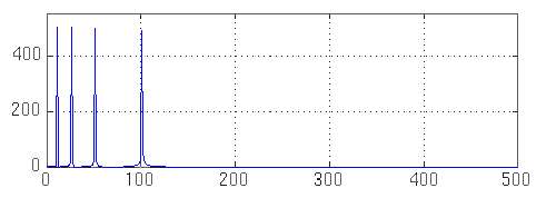
And for a non-stationary signal:
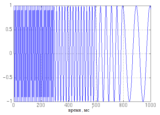
Fourier transform will be:
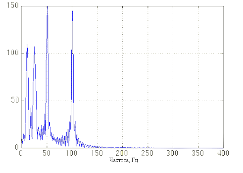
Thus, for two completely different signals, we get almost identical Fourier transforms (the smoothness of the Fourier transform graph for the second signal is not explained by the sudden change of frequency in this signal, and the difference in amplitude of different frequencies is explained by the fact that these frequencies acted for different times on the considered signal segment).
Thus, the Fourier transform in its essence cannot distinguish a stationary signal from a non-stationary signal, which is a big problem for its applicability.
Another tool for spectral analysis is the Fourier window transform (Short-Time Fourier transform), which is a type of Fourier transform and is defined as follows:
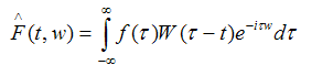
where W (Tau-t) is some window function.
Usually, a Gaussian, a Hamming window, a Hanna window or a Kaiser window are used as the window function.
The windowed Fourier transform, unlike the usual Fourier transform, is already a function of time, frequency, and amplitude. That is, it allows to obtain the characteristic of the frequency distribution of the signal (with amplitude) in time.
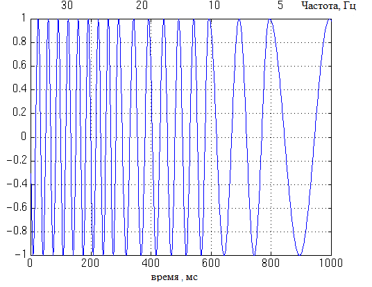
Consider the following non-stationary signal:
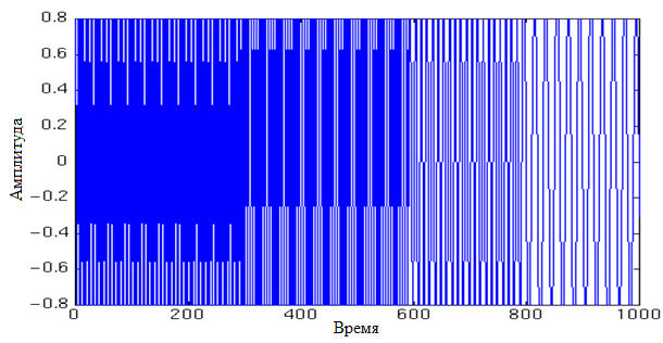
This signal is stationary every 250 ms (it has a frequency of 300 Hz on the first segment of the length of 250 ms, 200 Hz on the second, 100 Hz on the third, and 50 Hz on the fourth).
The three-dimensional (time, frequency and amplitude) graph of the window Fourier transform will look like this:
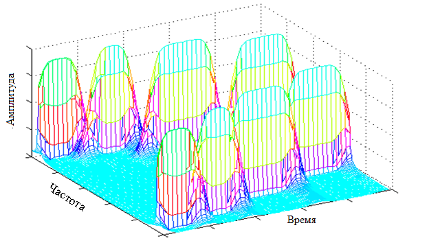
(the symmetry of the graph is explained by the fact that the Fourier transforms (including the window Fourier transforms) are symmetrical for any signal)
On this graph, we can see four pronounced maxima, which correspond to the frequencies present in the signal. The most important thing is that, unlike the usual Fourier transform, we get the values of frequencies relative to the time axis, that is, we get the time-frequency response of the signal.
But the main problem in using the window Fourier transform to obtain the time-frequency characteristics of a signal is the so-called Heisenberg uncertainty principle , which arises for the parameters of time and frequency of a signal.
The principle of uncertainty is based on the fact that it is impossible to say exactly what frequency is present in a signal at a given time (you can only talk about the frequency range) and it’s not possible to say at which exact time the frequency is present in the signal (you can only speak about a time period) .
This raises the problem of resolution. The resolution of the window Fourier transform can be adjusted using the width of the window.
A windowed Fourier transform with a narrow Gaussian window with a scale (reciprocal to the width of the window) 0.01 will look like this:
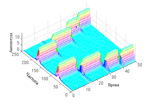
As can be seen, the resulting Fourier transform has good accuracy with respect to time and poor accuracy with respect to frequency (each maximum occupies a certain range of frequencies).
When using a wider Gaussian window with a scale of 0.00001, the window transform will look like:
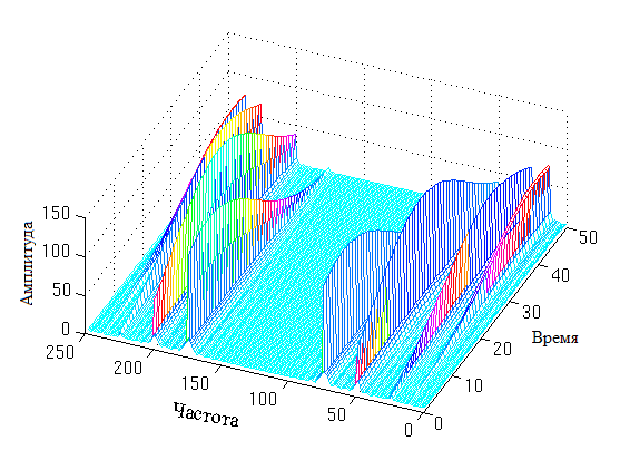
It is seen that in this case we get high accuracy with respect to frequency, but at the same time very low accuracy with respect to time.
We can assume that the ordinary Fourier transform is a window Fourier transform with a window width to infinity.
Thus, by increasing the width of the window (reducing its resolution), we increase the accuracy relative to frequency and decrease the accuracy relative to time.
What then to choose the value of the width of the window in order to achieve the optimal ratio of accuracy? The wavelet transform answers this question.
The wavelet transform was created as a tool that solves the problem of Heisenberg uncertainty for constructing the time-frequency characteristics of a signal.
Wavelet transform of the signal f (t) has the form:

where Tau is the time shift, S is the scale, and Psi * is the mother wavelet.
The concept of a wavelet means a wave that passes through a signal and is a window of a certain width (scale) for a certain location in time, during (forgive the tautology) the integration of the signal.
Maternal wavelet is a function that is a prototype for all windows that will be generated during wavelet transform.
The time shift controls the movement of the generated windows along the time component of the signal.
The concept of scale is inverse to the concept of window width. The smaller the width of the window, the larger the scale, that is, the window captures a smaller part of the signal and the signal is integrated more “in detail”.
The larger the width of the window, the smaller the scale, that is, the window captures most of the signal and the signal, respectively, integrates less “in detail”.
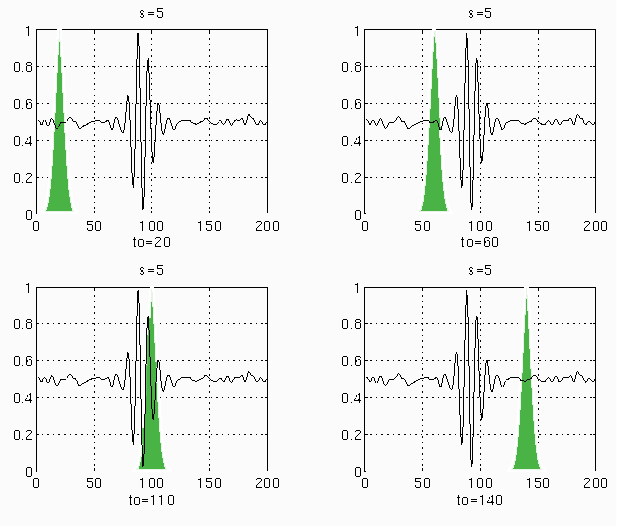
Let us describe the process of wavelet transformation (a Gaoussian is used as the maternal wavelet) of a certain continuous signal, which acted for a certain period of time (0-200ms) with a normalized amplitude (0-1):
1. Calculate the integral under the initial conditions Tau = 0 and S = 1;
a) the parameter Tau (i) = Tau (i-1) + e increases by some sufficiently small number e and the integral is calculated. Runs until Tau (i) becomes 200ms (end of signal).

2. The parameter S = 5 changes, the Tau value is again set to the starting point of the signal (Tau = 0);
a) the parameter Tau (i) = Tau (i-1) + e increases by some sufficiently small number e and the integral is calculated. Runs until Tau (i) becomes 200ms (end of signal).
The integrals for the parameter values S = 20, S = 50, etc. are calculated in the same way.
As a result of the described process, we obtain the calculated values of the integrals of the function for each scale at each time point.
Thus, we obtain a three-dimensional representation of the signal with components: scale, time, and amplitude (the values of the calculated integrals).
Consider the following non-stationary signal:
The wavelet transform for such a signal will be:
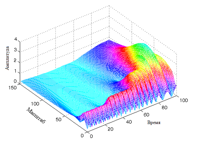
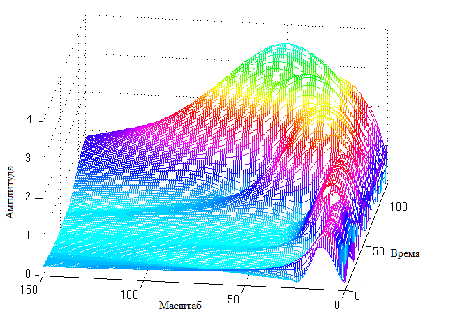
Thus, the wavelet transform, unlike the window Fourier transform, which has a constant scale at any time for all frequencies, has a better time representation and a worse frequency representation at low frequencies of the signal and a better frequency representation with a worse time representation at high frequencies of the signal .
The figures clearly show that the obtained wavelet transform is more detailed in time in the region of high scale values (low frequencies) and less detailed in the region of low scale values (high frequencies).
From this it follows that the wavelet transform makes it possible to reduce the influence of the Heisenberg uncertainty principle on the received time-frequency representation of the signal. With it, low frequencies have a more detailed presentation regarding time, and high frequencies refer to frequency.
References: Wavelet-tutorial
Recently, articles began to appear on the Habré in one way or another related to the analysis and processing of signals and images (for example, Detecting stable image features: the SURF method , Integral representation of images from BigObfuscator ), in connection with which I would like to briefly highlight such a tool for analysis signals as a wavelet transform.
In order to understand the meaning of wavelet analysis, let's start quite far away. This article describes the mathematical meaning (in simple terms) of the wavelet transform, I will tell you about the applicability and its discrete version later.
Spectral analysis is one of the signal processing methods that allows characterization of the frequency component of the measured signal.
')
Fourier transform
The main mathematical basis of spectral analysis is the Fourier transform , which relates the spatial or temporal signal (or some model of this signal) with its representation in the frequency domain.
The Fourier transform of the function f is an integral representation and is given by the following formula:
But the Fourier transform gives information only about the frequency that is present in the signal and does not give any information about the time interval at which this frequency is present in the signal.
Thus for the following stationary signal:
Fourier transform will be:
And for a non-stationary signal:
Fourier transform will be:
Thus, for two completely different signals, we get almost identical Fourier transforms (the smoothness of the Fourier transform graph for the second signal is not explained by the sudden change of frequency in this signal, and the difference in amplitude of different frequencies is explained by the fact that these frequencies acted for different times on the considered signal segment).
Thus, the Fourier transform in its essence cannot distinguish a stationary signal from a non-stationary signal, which is a big problem for its applicability.
Window Fourier Transform
Another tool for spectral analysis is the Fourier window transform (Short-Time Fourier transform), which is a type of Fourier transform and is defined as follows:
where W (Tau-t) is some window function.
Usually, a Gaussian, a Hamming window, a Hanna window or a Kaiser window are used as the window function.
The windowed Fourier transform, unlike the usual Fourier transform, is already a function of time, frequency, and amplitude. That is, it allows to obtain the characteristic of the frequency distribution of the signal (with amplitude) in time.
Consider the following non-stationary signal:
This signal is stationary every 250 ms (it has a frequency of 300 Hz on the first segment of the length of 250 ms, 200 Hz on the second, 100 Hz on the third, and 50 Hz on the fourth).
The three-dimensional (time, frequency and amplitude) graph of the window Fourier transform will look like this:
(the symmetry of the graph is explained by the fact that the Fourier transforms (including the window Fourier transforms) are symmetrical for any signal)
On this graph, we can see four pronounced maxima, which correspond to the frequencies present in the signal. The most important thing is that, unlike the usual Fourier transform, we get the values of frequencies relative to the time axis, that is, we get the time-frequency response of the signal.
But the main problem in using the window Fourier transform to obtain the time-frequency characteristics of a signal is the so-called Heisenberg uncertainty principle , which arises for the parameters of time and frequency of a signal.
The principle of uncertainty is based on the fact that it is impossible to say exactly what frequency is present in a signal at a given time (you can only talk about the frequency range) and it’s not possible to say at which exact time the frequency is present in the signal (you can only speak about a time period) .
This raises the problem of resolution. The resolution of the window Fourier transform can be adjusted using the width of the window.
A windowed Fourier transform with a narrow Gaussian window with a scale (reciprocal to the width of the window) 0.01 will look like this:
As can be seen, the resulting Fourier transform has good accuracy with respect to time and poor accuracy with respect to frequency (each maximum occupies a certain range of frequencies).
When using a wider Gaussian window with a scale of 0.00001, the window transform will look like:
It is seen that in this case we get high accuracy with respect to frequency, but at the same time very low accuracy with respect to time.
We can assume that the ordinary Fourier transform is a window Fourier transform with a window width to infinity.
Thus, by increasing the width of the window (reducing its resolution), we increase the accuracy relative to frequency and decrease the accuracy relative to time.
What then to choose the value of the width of the window in order to achieve the optimal ratio of accuracy? The wavelet transform answers this question.
Wavelet transform
The wavelet transform was created as a tool that solves the problem of Heisenberg uncertainty for constructing the time-frequency characteristics of a signal.
Wavelet transform of the signal f (t) has the form:
where Tau is the time shift, S is the scale, and Psi * is the mother wavelet.
The concept of a wavelet means a wave that passes through a signal and is a window of a certain width (scale) for a certain location in time, during (forgive the tautology) the integration of the signal.
Maternal wavelet is a function that is a prototype for all windows that will be generated during wavelet transform.
The time shift controls the movement of the generated windows along the time component of the signal.
The concept of scale is inverse to the concept of window width. The smaller the width of the window, the larger the scale, that is, the window captures a smaller part of the signal and the signal is integrated more “in detail”.
The larger the width of the window, the smaller the scale, that is, the window captures most of the signal and the signal, respectively, integrates less “in detail”.
Let us describe the process of wavelet transformation (a Gaoussian is used as the maternal wavelet) of a certain continuous signal, which acted for a certain period of time (0-200ms) with a normalized amplitude (0-1):
1. Calculate the integral under the initial conditions Tau = 0 and S = 1;
a) the parameter Tau (i) = Tau (i-1) + e increases by some sufficiently small number e and the integral is calculated. Runs until Tau (i) becomes 200ms (end of signal).
2. The parameter S = 5 changes, the Tau value is again set to the starting point of the signal (Tau = 0);
a) the parameter Tau (i) = Tau (i-1) + e increases by some sufficiently small number e and the integral is calculated. Runs until Tau (i) becomes 200ms (end of signal).
The integrals for the parameter values S = 20, S = 50, etc. are calculated in the same way.
As a result of the described process, we obtain the calculated values of the integrals of the function for each scale at each time point.
Thus, we obtain a three-dimensional representation of the signal with components: scale, time, and amplitude (the values of the calculated integrals).
Consider the following non-stationary signal:
The wavelet transform for such a signal will be:
Thus, the wavelet transform, unlike the window Fourier transform, which has a constant scale at any time for all frequencies, has a better time representation and a worse frequency representation at low frequencies of the signal and a better frequency representation with a worse time representation at high frequencies of the signal .
The figures clearly show that the obtained wavelet transform is more detailed in time in the region of high scale values (low frequencies) and less detailed in the region of low scale values (high frequencies).
From this it follows that the wavelet transform makes it possible to reduce the influence of the Heisenberg uncertainty principle on the received time-frequency representation of the signal. With it, low frequencies have a more detailed presentation regarding time, and high frequencies refer to frequency.
References: Wavelet-tutorial
Source: https://habr.com/ru/post/103899/
All Articles