JPEG decoding for dummies
UPD. Was forced to remove monospace formatting. One fine day, habraparser stopped understanding formatting inside the pre and code tags. The whole text turned to mush. Administration habr could not help me. Now uneven, but at least readable.
[FF D8]
Have you ever wanted to know how a jpg file works? Now we will understand! Warm up your favorite compiler and hex editor, we will decode it:
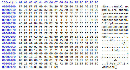
Specially took a smaller picture. This is a familiar, but strongly squeezed Google favicon:
')
Immediately I warn you that the description is simplified, and the information provided is not complete, but then it will be easy to understand the specification.
Even without knowing how the encoding happens, we can already extract something from the file.
[FF D8] - the start marker. It is always at the beginning of all jpg-files.
Following are the bytes [FF FE] . This is a marker indicating the beginning of the section with a comment. The next 2 bytes [00 04] is the section length (including these 2 bytes). So in the next two [3A 29] - the comment itself. These are the character codes ":" and ")", i.e. normal emoticon. You can see it in the first line of the right side of the hex editor.
Very briefly in steps:

I recall that each block Y ij , Cb ij , Cr ij is a matrix of DCT coefficients encoded by Huffman codes. In the file they are arranged in this order:Y 00 Y 10 Y 01 Y 11 Cb 00 Cr 00 Y 20
After we have extracted the comment, it will be easy to understand that:
FF D8 FF FE 00 04 3A 29 FF DB 00 43 00 A0 6E 78
8C 78 64 A0 8C 82 8C B4 AA A0 BE F0 FF FF F0 DC
FF FF FF FF FF FF FF FF FF FF FF FF FF FF FF FF
FF FF FF FF FF FF FF FF FF FF FF FF FF FF FF FF FF FF FF
FF FF FF FF FF FF FF FF FF FF FF FF FF FF FF FF FF DB 00
43 01 AA B4 B4 F0 D2 F0 FF FF FF FF FF FF FF FF
FF FF FF FF FF FF FF FF FF FF FF FF FF FF FF FF FF FF FF
FF FF FF FF FF FF FF FF FF FF FF FF FF FF FF FF FF FF FF
FF FF FF FF FF FF FF FF FF FF FF FF FF FF FF FF FF FF FF
FF FF FF C0 00 11 08 00 10 00 10 03 01 22 00 02
11 01 03 11 01 FF C4 00 15 00 01 01 00 00 00 00
00 00 00 00 00 00 00 00 00 00 03 02 FF C4 00 1A
10 01 00 02 03 01 00 00 00 00 00 00 00 00 00 00
00 01 00 12 02 11 31 21 FF C4 00 15 01 01 01 00
00 00 00 00 00 00 00 00 00 00 00 00 00 00 01 FF
C4 00 16 11 01 01 01 00 00 00 00 00 00 00 00 00
00 00 00 00 11 00 01 FF DA 00 0C 03 01 00 02 11
03 11 00 3F 00 AE E7 61 F2 1B D5 22 85 5D 04 3C
82 C8 48 B1 DC BF FF D9
FF DB 00 43 00 A0 6E 78
8C 78 64 A0 8C 82 8C B4 AA A0 BE F0 FF FF F0 DC
FF FF FF FF FF FF FF FF FF FF FF FF FF FF FF FF
FF FF FF FF FF FF FF FF FF FF FF FF FF FF FF FF FF FF FF
FF FF FF FF FF FF FF FF FF FF FF FF FF FF FF
The section header always takes 3 bytes. In our case it is [00 43 00]. The header consists of:
[00 43] Length: 0x43 = 67 bytes
[0_] The length of the values in the table: 0 (0 - 1 byte, 1 - 2 bytes)
[_0] Table ID: 0
The remaining 64 bytes need to fill the table 8x8.
[A0 6E 64 A0 F0 FF FF FF]
[78 78 8C BE FF FF FF FF]
[8C 82 A0 F0 FF FF FF FF]
[8C AA DC FF FF FF FF]
[B4 DC FF FF FF FF FF]
[F0 FF FF FF FF FF FF]
[FF FF FF FF FF FF FF]
[FF FF FF FF FF FF FF]
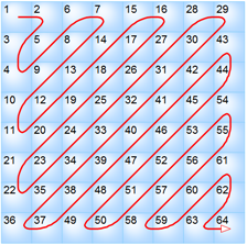
Look at the order in which the table values are filled. This order is called zigzag order:
This marker is called SOF0, and means that the image is encoded with the base method. It is very common. But the progressive-method familiar to you is no less popular on the Internet, when you first load an image with a low resolution, and then a normal picture. This allows you to understand what is shown there, without waiting for the full load. The specification defines a few more, as it seems to me, not very common methods.
FF C0 00 11 08 00 10 00 10 03 01 22 00 02
11 01 03 11 01
[00 11] Length: 17 bytes.
[08] Precision: 8 bits. In the base method is always 8. As I understand it, this is the width of the channel values.
[00 10] The height of the pattern: 0x10 = 16
[00 10] Pattern width: 0x10 = 16
[03] Number of components: 3. Most often it is Y, Cb, Cr.
1st component:
[01] ID: 1
[2_] Horizontal thinning (H 1 ): 2
[_2] Vertical thinning (V 1 ): 2
[00] Quantization Table ID: 0
2nd component:
[02] ID: 2
[1_] Horizontal thinning (H 2 ): 1
[_1] Vertical thinning (V 2 ): 1
[01] Quantization table ID: 1
3rd component:
[03] ID: 3
[1_] Horizontal thinning (H 3 ): 1
[_1] Vertical thinning (V 3 ): 1
[01] Quantization table ID: 1
Now look at how to determine how thinned the image is. FindH max = 2 and V max = 2. Channel i will be cut in H max / H i times horizontally and V max / V i times vertically.
This section stores codes and values obtained by Huffman coding .
FF C4 00 15 00 01 01 00 00 00 00
00 00 00 00 00 00 00 00 00 00 03 02
[00 15] length: 21 bytes.
[0_] class: 0 (0 is a table of DC coefficients, 1 is a table of AC coefficients).
[_0] table ID: 0
The length of the Huffman code: 1 2 3 4 5 6 7 8 9 10 11 12 13 14 15 16
Number of codes: [01 01 00 00 00 00 00 00 00 00 00 00 00 00 00 00]
The number of codes means the number of codes of this length. Note that the section stores only the length of the codes, not the codes themselves. We have to find the codes ourselves. So, we have one code of length 1 and one - length 2. Total 2 codes, there are no more codes in this table.
Each code is associated with a value; they are listed next in the file. Values are single-byte, so we read 2 bytes.
[03] - the value of the 1st code.
[02] - the value of the 2nd code.
Further in the file you can see 3 more markers [FF C4], I will skip the analysis of the corresponding sections, it is similar to the above.
We need to build a binary tree on the table that we got in the DHT section. And already on this tree, we learn each code. Values are added in the order shown in the table. The algorithm is simple: in whatever node we are, we always try to add value to the left branch. And if she is busy, then right. And if there is no place there, then we return to the level above, and try from there. You need to stop at a level equal to the length of the code. The left branches correspond to thevalue 0 , the right - 1 .
Comment:
No need to start from the top every time. Added value - go back one level. Does the right branch exist? If yes, go up again. If not, create the right branch and go there. Then, from this point, start the search to add the next value.
Trees for all tables in this example:
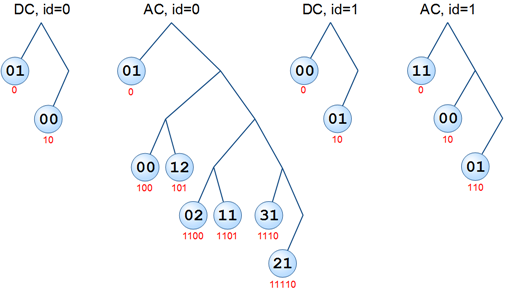
UPD (thanks to anarsoul ): At the nodes of the first tree (DC, id = 0), the values 0x03 and 0x02 should be
In the circles - the values of the codes, under the circles - the codes themselves (I will explain that we got them by going from the top to each node). It is with such codes (this and other tables) that the very content of the picture is encoded.
Byte [DA] in the marker means - "YES! Finally, we went directly to the analysis section of the encoded image! ". However, the section is symbolically called SOS.
& nbsp FF DA 00 0C 03 01 00 02 11
03 11 00 3F 00
[00 0C] The length of the header part (and not the entire section): 12 bytes.
[03] The number of scan components. We have 3, one for Y, Cb, Cr.
1st component:
[01] Image component number: 1 (Y)
[0_] Huffman table ID for DC coefficients: 0
[_0] Huffman table ID for AC coefficients: 0
2nd component:
[02] Image component number: 2 (Cb)
[1_] Huffman table identifier for DC coefficients: 1
[_1] Huffman table identifier for AC coefficients: 1
3rd component:
[03] Image component number: 3 (Cr)
[1_] Huffman table identifier for DC coefficients: 1
[_1] Huffman table identifier for AC coefficients: 1
These components alternate cyclically.
[00], [3F], [00] You can read about these bytes in the specification.
This ends the header part, from here to the end (marker [FF D9]) encoded data.
[AE] [E7] [61] [F2] [1B]
101011101110011101100001111100100
Finding DC coefficient.
1. We read a sequence of bits (if we meet 2 bytes [FF 00], then this is not a marker, but simply a byte [FF]) . After each bit, we move along the Huffman tree (with the corresponding identifier) along the 0 or 1 branch, depending on the read bit. We stop if we are in the final node.
10 1011101110011101100001111100100
2. Take the value of the node. If it is 0, then the coefficient is 0, write to the table and go on to reading other coefficients. In our case, 02. This value is the length of the coefficient in bits. That is, we read the next 2 bits, this will be the coefficient.
10 10 11101110011101100001111100100
3. If the first digit of the value in binary representation is 1, then leave it as it is: DC_coef = value. Otherwise, convert:DC_coef = value-2 is the length of the value +1 . Write the coefficient in the table at the beginning of the zigzag - the upper left corner.
Finding AC coefficients.
1. Similar to p. 1, finding the DC coefficient. We continue to read the sequence:
10 10 1110 1110011101100001111100100
2. Take the value of the node. If it is 0, this means that the remaining values of the matrix must be filled with zeros. Further the next matrix is already encoded. The first few who have read this far and have written about this to me in PM will get a plus in karma. In our case, the value of the node: 0x31.
The first nibble: 0x3 is exactly the number of zeros we need to add to the matrix. These are 3 zero coefficients.
The second nibble: 0x1 is the length of the coefficient in bits. We read the next bit.
10 10 1110 1 110011101100001111100100
3. Similar to p. 3 of finding the DC-coefficient.
As you already understood, it is necessary to read the AC-coefficients until we stumble upon the zero code value, or until the matrix is filled.
In our case, we get:
10 10 1110 1 1100 11 101 10 0 0 0 1 11110 0 100
and matrix:
[2 0 3 0 0 0 0 0]
[0 1 2 0 0 0 0 0]
[0 -1 -1 0 0 0 0 0]
[1 0 0 0 0 0 0 0]
[0 0 0 0 0 0 0 0]
[0 0 0 0 0 0 0 0]
[0 0 0 0 0 0 0 0]
[0 0 0 0 0 0 0 0]
Have you noticed that the values are filled in the same zigzag order?
The reason for using such an order is simple - since the larger the values of v and u, the smaller the significance of the coefficient S vu in the discrete-cosine transform. Therefore, at high compression ratios, minor coefficients are zeroed out, thereby reducing the file size.
Similarly, we get another 3 matrix Y-channel ...
[-4 1 1 1 0 0 0 0] [5 -1 1 0 0 0 0 0]
[0 0 1 0 0 0 0 0] [-1 -2 -1 0 0 0 0 0]
[0 -1 0 0 0 0 0 0] [0 -1 0 0 0 0 0]
[0 0 0 0 0 0 0] [-1 0 0 0 0 0 0]
[0 0 0 0 0 0 0] [0 0 0 0 0 0 0]
[0 0 0 0 0 0 0] [0 0 0 0 0 0 0]
[0 0 0 0 0 0 0] [0 0 0 0 0 0 0]
[0 0 0 0 0 0 0] [0 0 0 0 0 0 0]
[-4 2 2 1 0 0 0 0]
[-1 0 -1 0 0 0 0 0]
[-1 -1 0 0 0 0 0 0]
[0 0 0 0 0 0 0 0]
[0 0 0 0 0 0 0 0]
[0 0 0 0 0 0 0 0]
[0 0 0 0 0 0 0 0]
[0 0 0 0 0 0 0 0]
Oh, I forgot to say that the coded DC coefficients are not the DC coefficients themselves, but their differences between the coefficients of the previous table (of the same channel)! It is necessary to correct the matrix:
DC for the 2nd: 2 + (-4) = -2
DC for the 3rd: -2 + 5 = 3
DC for the 4th: 3 + (-4) = -1
[-2 1 1 1 0 0 0 0] [3 -1 1 0 0 0 0 0] [-1 2 2 1 0 0 0 0]
………
Now order. This rule is valid until the end of the file.
... and on the matrix for Cb and Cr:
[-1 0 0 0 0 0 0] [0 0 0 0 0 0 0]
[1 1 0 0 0 0 0 0] [1 -1 0 0 0 0 0]
[0 0 0 0 0 0 0] [1 0 0 0 0 0 0]
[0 0 0 0 0 0 0] [0 0 0 0 0 0 0]
[0 0 0 0 0 0 0] [0 0 0 0 0 0 0]
[0 0 0 0 0 0 0] [0 0 0 0 0 0 0]
[0 0 0 0 0 0 0] [0 0 0 0 0 0 0]
[0 0 0 0 0 0 0] [0 0 0 0 0 0 0]
Since there is only one matrix, DC coefficients can not touch.
Do you remember that the matrix passes the quantization stage? Matrix elements need to be multiplied by the elements of the quantization matrix. It remains to choose the right one. First, we scanned the first component, its image component = 1. The image component with this identifier uses the quantization matrix 0 (we have the first of the two). So, after multiplication:
[320 0 300 0 0 0 0 0]
[0 120 280 0 0 0 0 0]
[0 -130 -160 0 0 0 0 0]
[140 0 0 0 0 0 0 0]
[0 0 0 0 0 0 0 0]
[0 0 0 0 0 0 0 0]
[0 0 0 0 0 0 0 0]
[0 0 0 0 0 0 0 0]
Similarly, we get another 3 matrix Y-channel ...
[-320 110 100 160 0 0 0 0] [480 -110 100 0 0 0 0]
[0 0 140 0 0 0 0 0] [-120 -240 -140 0 0 0 0 0]
[0 -130 0 0 0 0 0 0] [0 -130 0 0 0 0 0 0]
[0 0 0 0 0 0 0] [-140 0 0 0 0 0 0]
[0 0 0 0 0 0 0] [0 0 0 0 0 0 0]
[0 0 0 0 0 0 0] [0 0 0 0 0 0 0]
[0 0 0 0 0 0 0] [0 0 0 0 0 0 0]
[0 0 0 0 0 0 0] [0 0 0 0 0 0 0]
[-160 220 200 160 0 0 0 0]
[-120 0 -140 0 0 0 0 0]
[-140 -130 0 0 0 0 0 0]
[0 0 0 0 0 0 0 0]
[0 0 0 0 0 0 0 0]
[0 0 0 0 0 0 0 0]
[0 0 0 0 0 0 0 0]
[0 0 0 0 0 0 0 0]
... and on the matrix for Cb and Cr.
[-170 0 0 0 0 0 0 0] [0 0 0 0 0 0 0]
[180 210 0 0 0 0 0 0] [180 -210 0 0 0 0 0 0]
[0 0 0 0 0 0 0] [240 0 0 0 0 0 0]
[0 0 0 0 0 0 0] [0 0 0 0 0 0 0]
[0 0 0 0 0 0 0] [0 0 0 0 0 0 0]
[0 0 0 0 0 0 0] [0 0 0 0 0 0 0]
[0 0 0 0 0 0 0] [0 0 0 0 0 0 0]
[0 0 0 0 0 0 0] [0 0 0 0 0 0 0]
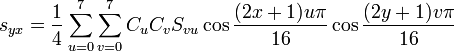

The formula should not deliver difficulties *. S vu is our derived coefficient matrix. u is a column, v is a string. s yx - directly the values of the channels.
* Generally speaking, this is not entirely true. When I was able to decode and display a 16x16 image on the screen, I took a 600x600 image (by the way, it was the cover of my favorite album Mind.In.A.Box - Lost Alone). It didn't work out right away - various bugs surfaced. Soon I could admire the correctly loaded picture. Only very upset the download speed. I still remember, it took 7 seconds. But it is not surprising if you thoughtlessly use the above formula, then to calculate one channel of one pixel you will need to find 128 cosines, 768 multiplications, and some additions. Just think - almost a thousand difficult operations on just one channel of one pixel! Fortunately, there is room for optimizing (after long experiments, I reduced the download time to the 15ms timer accuracy limit, and after that I changed the image to a photo with a 25 times larger area. Perhaps I will write about this in a separate article).
I will write the result of calculating only the first matrix of the channel Y (values are rounded):
[138 92 27 -17 -17 28 93 139]
[136 82 5 -51 -55 -8 61 111]
[143 80 -9 -77 -89 -41 32 32 86]
[157 95 6 -62 -76 -33 36 86]
[147 103 37 -12 -21 11 62 100]
[87 72 50 36 37 55 79 95]
[-10 5 31 56 71 73 68 62]
[-87 -50 6 56 79 72 48 29]
and 2 remaining:
Cb cr
[60 52 38 20 0 -18 -32 -40] [19 27 41 60 80 99 113 120]
[48 41 29 13 -3 -19 -31 -37] [0 6 18 34 51 66 78 85]
[25 20 12 2 -9 -19 -27 -32] [-27 -22 -14 -4 7 17 25 30]
[-4 -6 -9 -13 -17 -20 -23 -25] [-43 -41 -38 -34 -30 -27 -24 -22]
[-37 -35 -33 -29 -25 -21 -18 -17] [-35 -36 -39 -43 -47 -51 -53 -55]
[-67 -63 -55 -44 -33 -22 -14 -10] [-5 -9 -17 -28 -39 -50 -58 -62]
[-90 -84 -71 -56 -39 -23 -11 -4] [32 26 14 -1 -18 -34 -46 -53]
[-102 -95 -81 -62 -42 -23 -9 -1] [58 50 36 18 -2 -20 -34 -42]
And now ... a mini test!
What to do next?
R = Y + 1.402 * Cr
G = Y - 0.34414 * Cb - 0.71414 * Cr
B = Y + 1.772 * Cb
Do not forget to add 128 each. If the values fall outside the interval [0, 255], then assign the boundary values. The formula is simple, but it also erases the share of CPU time.
Here are the resulting tables for the channels R, G, B for the left upper square 8x8 of our example:
255 248 194 148 169 215 255 255
255 238 172 115 130 178 255 255
255 208 127 59 64 112 208 255
255 223 143 74 77 120 211 255
237 192 133 83 85 118 184 222
177 161 146 132 145 162 201 217
56 73 101 126 144 147 147 141
0 17 76 126 153 146 127 108
231 185 117 72 67 113 171 217
229 175 95 39 28 76 139 189
254 192 100 31 15 63 131 185
255 207 115 46 28 71 134 185
255 241 175 125 112 145 145 193 230
226 210 187 173 172 189 209 225
149 166 191 216 229 232 225 220
72 110 166 216 238 231 206 186
255 255 249 203 178 224 255 255
255 255 226 170 140 187 224 255
255 255 192 123 91 138 184 238
255 255 208 139 103 146 188 239
255 255 202 152 128 161 194 232
255 244 215 200 188 205 210 227
108 125 148 172 182 184 172 167
31 69 122 172 191 183 153 134
In general, I am not an expert on JPEG, so I can hardly answer all the questions. Just when I was writing my decoder, I often had to face various incomprehensible problems. And when the image was displayed incorrectly, I did not know where I had made a mistake. Maybe he incorrectly interpreted the bits, and maybe incorrectly used DCT. There was a lack of a step-by-step example, so I hope this article will help in writing a decoder. I think it covers the description of the base method, but still it is impossible to do only by it. I offer you links that helped me:
ru.wikipedia.org/JPEG - for superficial acquaintance.
en.wikipedia.org/JPEG is a much more sensible article on encoding / decoding processes.
JPEG Standard (JPEG ISO / IEC 10918-1 ITU-T Recommendation T.81) - can not do without the 186-page specification. But there is no reason to panic - three quarters are flowcharts and applications.
impulseadventure.com/photo - Good detailed articles. By examples, I figured out how to build Huffman trees and use them when reading the relevant section.
JPEGsnoop - On the same site there is a great utility that pulls out all the information of a jpeg-file.
[FF D9]
[FF D8]
Have you ever wanted to know how a jpg file works? Now we will understand! Warm up your favorite compiler and hex editor, we will decode it:
Specially took a smaller picture. This is a familiar, but strongly squeezed Google favicon:
')
Immediately I warn you that the description is simplified, and the information provided is not complete, but then it will be easy to understand the specification.
Even without knowing how the encoding happens, we can already extract something from the file.
[FF D8] - the start marker. It is always at the beginning of all jpg-files.
Following are the bytes [FF FE] . This is a marker indicating the beginning of the section with a comment. The next 2 bytes [00 04] is the section length (including these 2 bytes). So in the next two [3A 29] - the comment itself. These are the character codes ":" and ")", i.e. normal emoticon. You can see it in the first line of the right side of the hex editor.
A bit of theory
Very briefly in steps:
- Normally, the image is converted from RGB color space to YCbCr .
- Often the channels Cb and Cr are thinned, that is, the average value is assigned to a block of pixels. For example, after thinning 2 times vertically and horizontally, the pixels will have the following correspondence:

- Then the channel values are divided into 8x8 blocks (everyone saw these small squares on a too compressed image).
- Each block is subjected to a discrete cosine transform (DCT) , which is a kind of discrete Fourier transform . Get the 8x8 matrix of coefficients. Moreover, the upper left coefficient is called the DC coefficient (it is the most important and is the average value of all values), and the remaining 63 coefficient is the AC coefficients.
- The resulting coefficients are quantized, i.e. each is multiplied by the quantization matrix coefficient (each encoder usually uses its own quantization matrix).
- Then they are encoded by Huffman codes .
I recall that each block Y ij , Cb ij , Cr ij is a matrix of DCT coefficients encoded by Huffman codes. In the file they are arranged in this order:
Reading file
After we have extracted the comment, it will be easy to understand that:
- The file is divided into sectors preceded by markers.
- Markers are 2 bytes long, with the first byte [FF].
- Almost all sectors store their length in the next 2 bytes after the marker.
FF D8 FF FE 00 04 3A 29 FF DB 00 43 00 A0 6E 78
8C 78 64 A0 8C 82 8C B4 AA A0 BE F0 FF FF F0 DC
FF FF FF FF FF FF FF FF FF FF FF FF FF FF FF FF
FF FF FF FF FF FF FF FF FF FF FF FF FF FF FF FF FF FF FF
FF FF FF FF FF FF FF FF FF FF FF FF FF FF FF FF FF DB 00
43 01 AA B4 B4 F0 D2 F0 FF FF FF FF FF FF FF FF
FF FF FF FF FF FF FF FF FF FF FF FF FF FF FF FF FF FF FF
FF FF FF FF FF FF FF FF FF FF FF FF FF FF FF FF FF FF FF
FF FF FF FF FF FF FF FF FF FF FF FF FF FF FF FF FF FF FF
FF FF FF C0 00 11 08 00 10 00 10 03 01 22 00 02
11 01 03 11 01 FF C4 00 15 00 01 01 00 00 00 00
00 00 00 00 00 00 00 00 00 00 03 02 FF C4 00 1A
10 01 00 02 03 01 00 00 00 00 00 00 00 00 00 00
00 01 00 12 02 11 31 21 FF C4 00 15 01 01 01 00
00 00 00 00 00 00 00 00 00 00 00 00 00 00 01 FF
C4 00 16 11 01 01 01 00 00 00 00 00 00 00 00 00
00 00 00 00 11 00 01 FF DA 00 0C 03 01 00 02 11
03 11 00 3F 00 AE E7 61 F2 1B D5 22 85 5D 04 3C
82 C8 48 B1 DC BF FF D9
Marker [FF DB]: DQT - quantization table.
FF DB 00 43 00 A0 6E 78
8C 78 64 A0 8C 82 8C B4 AA A0 BE F0 FF FF F0 DC
FF FF FF FF FF FF FF FF FF FF FF FF FF FF FF FF
FF FF FF FF FF FF FF FF FF FF FF FF FF FF FF FF FF FF FF
FF FF FF FF FF FF FF FF FF FF FF FF FF FF FF
The section header always takes 3 bytes. In our case it is [00 43 00]. The header consists of:
[00 43] Length: 0x43 = 67 bytes
[0_] The length of the values in the table: 0 (0 - 1 byte, 1 - 2 bytes)
[_0] Table ID: 0
The remaining 64 bytes need to fill the table 8x8.
[A0 6E 64 A0 F0 FF FF FF]
[78 78 8C BE FF FF FF FF]
[8C 82 A0 F0 FF FF FF FF]
[8C AA DC FF FF FF FF]
[B4 DC FF FF FF FF FF]
[F0 FF FF FF FF FF FF]
[FF FF FF FF FF FF FF]
[FF FF FF FF FF FF FF]
Look at the order in which the table values are filled. This order is called zigzag order:
Marker [FF C0]: SOF0 - Baseline DCT
This marker is called SOF0, and means that the image is encoded with the base method. It is very common. But the progressive-method familiar to you is no less popular on the Internet, when you first load an image with a low resolution, and then a normal picture. This allows you to understand what is shown there, without waiting for the full load. The specification defines a few more, as it seems to me, not very common methods.
FF C0 00 11 08 00 10 00 10 03 01 22 00 02
11 01 03 11 01
[00 11] Length: 17 bytes.
[08] Precision: 8 bits. In the base method is always 8. As I understand it, this is the width of the channel values.
[00 10] The height of the pattern: 0x10 = 16
[00 10] Pattern width: 0x10 = 16
[03] Number of components: 3. Most often it is Y, Cb, Cr.
1st component:
[01] ID: 1
[2_] Horizontal thinning (H 1 ): 2
[_2] Vertical thinning (V 1 ): 2
[00] Quantization Table ID: 0
2nd component:
[02] ID: 2
[1_] Horizontal thinning (H 2 ): 1
[_1] Vertical thinning (V 2 ): 1
[01] Quantization table ID: 1
3rd component:
[03] ID: 3
[1_] Horizontal thinning (H 3 ): 1
[_1] Vertical thinning (V 3 ): 1
[01] Quantization table ID: 1
Now look at how to determine how thinned the image is. Find
Marker [FF C4]: DHT (Huffman table)
This section stores codes and values obtained by Huffman coding .
FF C4 00 15 00 01 01 00 00 00 00
00 00 00 00 00 00 00 00 00 00 03 02
[00 15] length: 21 bytes.
[0_] class: 0 (0 is a table of DC coefficients, 1 is a table of AC coefficients).
[_0] table ID: 0
The length of the Huffman code: 1 2 3 4 5 6 7 8 9 10 11 12 13 14 15 16
Number of codes: [01 01 00 00 00 00 00 00 00 00 00 00 00 00 00 00]
The number of codes means the number of codes of this length. Note that the section stores only the length of the codes, not the codes themselves. We have to find the codes ourselves. So, we have one code of length 1 and one - length 2. Total 2 codes, there are no more codes in this table.
Each code is associated with a value; they are listed next in the file. Values are single-byte, so we read 2 bytes.
[03] - the value of the 1st code.
[02] - the value of the 2nd code.
Further in the file you can see 3 more markers [FF C4], I will skip the analysis of the corresponding sections, it is similar to the above.
Building a tree of Huffman codes
We need to build a binary tree on the table that we got in the DHT section. And already on this tree, we learn each code. Values are added in the order shown in the table. The algorithm is simple: in whatever node we are, we always try to add value to the left branch. And if she is busy, then right. And if there is no place there, then we return to the level above, and try from there. You need to stop at a level equal to the length of the code. The left branches correspond to the
Comment:
No need to start from the top every time. Added value - go back one level. Does the right branch exist? If yes, go up again. If not, create the right branch and go there. Then, from this point, start the search to add the next value.
Trees for all tables in this example:
UPD (thanks to anarsoul ): At the nodes of the first tree (DC, id = 0), the values 0x03 and 0x02 should be
In the circles - the values of the codes, under the circles - the codes themselves (I will explain that we got them by going from the top to each node). It is with such codes (this and other tables) that the very content of the picture is encoded.
Marker [FF DA]: SOS (Start of Scan)
Byte [DA] in the marker means - "YES! Finally, we went directly to the analysis section of the encoded image! ". However, the section is symbolically called SOS.
& nbsp FF DA 00 0C 03 01 00 02 11
03 11 00 3F 00
[00 0C] The length of the header part (and not the entire section): 12 bytes.
[03] The number of scan components. We have 3, one for Y, Cb, Cr.
1st component:
[01] Image component number: 1 (Y)
[0_] Huffman table ID for DC coefficients: 0
[_0] Huffman table ID for AC coefficients: 0
2nd component:
[02] Image component number: 2 (Cb)
[1_] Huffman table identifier for DC coefficients: 1
[_1] Huffman table identifier for AC coefficients: 1
3rd component:
[03] Image component number: 3 (Cr)
[1_] Huffman table identifier for DC coefficients: 1
[_1] Huffman table identifier for AC coefficients: 1
These components alternate cyclically.
[00], [3F], [00] You can read about these bytes in the specification.
This ends the header part, from here to the end (marker [FF D9]) encoded data.
[AE] [E7] [61] [F2] [1B]
101011101110011101100001111100100
Finding DC coefficient.
1. We read a sequence of bits (if we meet 2 bytes [FF 00], then this is not a marker, but simply a byte [FF]) . After each bit, we move along the Huffman tree (with the corresponding identifier) along the 0 or 1 branch, depending on the read bit. We stop if we are in the final node.
10 1011101110011101100001111100100
2. Take the value of the node. If it is 0, then the coefficient is 0, write to the table and go on to reading other coefficients. In our case, 02. This value is the length of the coefficient in bits. That is, we read the next 2 bits, this will be the coefficient.
10 10 11101110011101100001111100100
3. If the first digit of the value in binary representation is 1, then leave it as it is: DC_coef = value. Otherwise, convert:
Finding AC coefficients.
1. Similar to p. 1, finding the DC coefficient. We continue to read the sequence:
10 10 1110 1110011101100001111100100
2. Take the value of the node. If it is 0, this means that the remaining values of the matrix must be filled with zeros. Further the next matrix is already encoded. The first few who have read this far and have written about this to me in PM will get a plus in karma. In our case, the value of the node: 0x31.
The first nibble: 0x3 is exactly the number of zeros we need to add to the matrix. These are 3 zero coefficients.
The second nibble: 0x1 is the length of the coefficient in bits. We read the next bit.
10 10 1110 1 110011101100001111100100
3. Similar to p. 3 of finding the DC-coefficient.
As you already understood, it is necessary to read the AC-coefficients until we stumble upon the zero code value, or until the matrix is filled.
In our case, we get:
10 10 1110 1 1100 11 101 10 0 0 0 1 11110 0 100
and matrix:
[2 0 3 0 0 0 0 0]
[0 1 2 0 0 0 0 0]
[0 -1 -1 0 0 0 0 0]
[1 0 0 0 0 0 0 0]
[0 0 0 0 0 0 0 0]
[0 0 0 0 0 0 0 0]
[0 0 0 0 0 0 0 0]
[0 0 0 0 0 0 0 0]
Have you noticed that the values are filled in the same zigzag order?
The reason for using such an order is simple - since the larger the values of v and u, the smaller the significance of the coefficient S vu in the discrete-cosine transform. Therefore, at high compression ratios, minor coefficients are zeroed out, thereby reducing the file size.
Similarly, we get another 3 matrix Y-channel ...
[-4 1 1 1 0 0 0 0] [5 -1 1 0 0 0 0 0]
[0 0 1 0 0 0 0 0] [-1 -2 -1 0 0 0 0 0]
[0 -1 0 0 0 0 0 0] [0 -1 0 0 0 0 0]
[0 0 0 0 0 0 0] [-1 0 0 0 0 0 0]
[0 0 0 0 0 0 0] [0 0 0 0 0 0 0]
[0 0 0 0 0 0 0] [0 0 0 0 0 0 0]
[0 0 0 0 0 0 0] [0 0 0 0 0 0 0]
[0 0 0 0 0 0 0] [0 0 0 0 0 0 0]
[-4 2 2 1 0 0 0 0]
[-1 0 -1 0 0 0 0 0]
[-1 -1 0 0 0 0 0 0]
[0 0 0 0 0 0 0 0]
[0 0 0 0 0 0 0 0]
[0 0 0 0 0 0 0 0]
[0 0 0 0 0 0 0 0]
[0 0 0 0 0 0 0 0]
Oh, I forgot to say that the coded DC coefficients are not the DC coefficients themselves, but their differences between the coefficients of the previous table (of the same channel)! It is necessary to correct the matrix:
DC for the 2nd: 2 + (-4) = -2
DC for the 3rd: -2 + 5 = 3
DC for the 4th: 3 + (-4) = -1
[-2 1 1 1 0 0 0 0] [3 -1 1 0 0 0 0 0] [-1 2 2 1 0 0 0 0]
………
Now order. This rule is valid until the end of the file.
... and on the matrix for Cb and Cr:
[-1 0 0 0 0 0 0] [0 0 0 0 0 0 0]
[1 1 0 0 0 0 0 0] [1 -1 0 0 0 0 0]
[0 0 0 0 0 0 0] [1 0 0 0 0 0 0]
[0 0 0 0 0 0 0] [0 0 0 0 0 0 0]
[0 0 0 0 0 0 0] [0 0 0 0 0 0 0]
[0 0 0 0 0 0 0] [0 0 0 0 0 0 0]
[0 0 0 0 0 0 0] [0 0 0 0 0 0 0]
[0 0 0 0 0 0 0] [0 0 0 0 0 0 0]
Since there is only one matrix, DC coefficients can not touch.
Calculations
Quantization
Do you remember that the matrix passes the quantization stage? Matrix elements need to be multiplied by the elements of the quantization matrix. It remains to choose the right one. First, we scanned the first component, its image component = 1. The image component with this identifier uses the quantization matrix 0 (we have the first of the two). So, after multiplication:
[320 0 300 0 0 0 0 0]
[0 120 280 0 0 0 0 0]
[0 -130 -160 0 0 0 0 0]
[140 0 0 0 0 0 0 0]
[0 0 0 0 0 0 0 0]
[0 0 0 0 0 0 0 0]
[0 0 0 0 0 0 0 0]
[0 0 0 0 0 0 0 0]
Similarly, we get another 3 matrix Y-channel ...
[-320 110 100 160 0 0 0 0] [480 -110 100 0 0 0 0]
[0 0 140 0 0 0 0 0] [-120 -240 -140 0 0 0 0 0]
[0 -130 0 0 0 0 0 0] [0 -130 0 0 0 0 0 0]
[0 0 0 0 0 0 0] [-140 0 0 0 0 0 0]
[0 0 0 0 0 0 0] [0 0 0 0 0 0 0]
[0 0 0 0 0 0 0] [0 0 0 0 0 0 0]
[0 0 0 0 0 0 0] [0 0 0 0 0 0 0]
[0 0 0 0 0 0 0] [0 0 0 0 0 0 0]
[-160 220 200 160 0 0 0 0]
[-120 0 -140 0 0 0 0 0]
[-140 -130 0 0 0 0 0 0]
[0 0 0 0 0 0 0 0]
[0 0 0 0 0 0 0 0]
[0 0 0 0 0 0 0 0]
[0 0 0 0 0 0 0 0]
[0 0 0 0 0 0 0 0]
... and on the matrix for Cb and Cr.
[-170 0 0 0 0 0 0 0] [0 0 0 0 0 0 0]
[180 210 0 0 0 0 0 0] [180 -210 0 0 0 0 0 0]
[0 0 0 0 0 0 0] [240 0 0 0 0 0 0]
[0 0 0 0 0 0 0] [0 0 0 0 0 0 0]
[0 0 0 0 0 0 0] [0 0 0 0 0 0 0]
[0 0 0 0 0 0 0] [0 0 0 0 0 0 0]
[0 0 0 0 0 0 0] [0 0 0 0 0 0 0]
[0 0 0 0 0 0 0] [0 0 0 0 0 0 0]
Inverse discrete cosine transform
The formula should not deliver difficulties *. S vu is our derived coefficient matrix. u is a column, v is a string. s yx - directly the values of the channels.
* Generally speaking, this is not entirely true. When I was able to decode and display a 16x16 image on the screen, I took a 600x600 image (by the way, it was the cover of my favorite album Mind.In.A.Box - Lost Alone). It didn't work out right away - various bugs surfaced. Soon I could admire the correctly loaded picture. Only very upset the download speed. I still remember, it took 7 seconds. But it is not surprising if you thoughtlessly use the above formula, then to calculate one channel of one pixel you will need to find 128 cosines, 768 multiplications, and some additions. Just think - almost a thousand difficult operations on just one channel of one pixel! Fortunately, there is room for optimizing (after long experiments, I reduced the download time to the 15ms timer accuracy limit, and after that I changed the image to a photo with a 25 times larger area. Perhaps I will write about this in a separate article).
I will write the result of calculating only the first matrix of the channel Y (values are rounded):
[138 92 27 -17 -17 28 93 139]
[136 82 5 -51 -55 -8 61 111]
[143 80 -9 -77 -89 -41 32 32 86]
[157 95 6 -62 -76 -33 36 86]
[147 103 37 -12 -21 11 62 100]
[87 72 50 36 37 55 79 95]
[-10 5 31 56 71 73 68 62]
[-87 -50 6 56 79 72 48 29]
and 2 remaining:
Cb cr
[60 52 38 20 0 -18 -32 -40] [19 27 41 60 80 99 113 120]
[48 41 29 13 -3 -19 -31 -37] [0 6 18 34 51 66 78 85]
[25 20 12 2 -9 -19 -27 -32] [-27 -22 -14 -4 7 17 25 30]
[-4 -6 -9 -13 -17 -20 -23 -25] [-43 -41 -38 -34 -30 -27 -24 -22]
[-37 -35 -33 -29 -25 -21 -18 -17] [-35 -36 -39 -43 -47 -51 -53 -55]
[-67 -63 -55 -44 -33 -22 -14 -10] [-5 -9 -17 -28 -39 -50 -58 -62]
[-90 -84 -71 -56 -39 -23 -11 -4] [32 26 14 -1 -18 -34 -46 -53]
[-102 -95 -81 -62 -42 -23 -9 -1] [58 50 36 18 -2 -20 -34 -42]
And now ... a mini test!
What to do next?
- Oh, let's go eat!
- Yes, I do not drive in, what I mean.
- Once the color values of YCbCr are obtained, it remains to convert to RGB, like this:
YCbCrToRGB (Y ij , Cb ij , Cr ij ), Y ij , Cb ij , Cr ij are our resulting matrices. - 4 matrices Y, and Cb and Cr each, since we thinned the channels and 4 pixels Y correspond to Cb and Cr each. Therefore, calculate as follows:
YCbCrToRGB (Y ij , Cb [i / 2] [j / 2] , Cr [i / 2] [j / 2] )
YCbCr to RGB
R = Y + 1.402 * Cr
G = Y - 0.34414 * Cb - 0.71414 * Cr
B = Y + 1.772 * Cb
Do not forget to add 128 each. If the values fall outside the interval [0, 255], then assign the boundary values. The formula is simple, but it also erases the share of CPU time.
Here are the resulting tables for the channels R, G, B for the left upper square 8x8 of our example:
255 248 194 148 169 215 255 255
255 238 172 115 130 178 255 255
255 208 127 59 64 112 208 255
255 223 143 74 77 120 211 255
237 192 133 83 85 118 184 222
177 161 146 132 145 162 201 217
56 73 101 126 144 147 147 141
0 17 76 126 153 146 127 108
231 185 117 72 67 113 171 217
229 175 95 39 28 76 139 189
254 192 100 31 15 63 131 185
255 207 115 46 28 71 134 185
255 241 175 125 112 145 145 193 230
226 210 187 173 172 189 209 225
149 166 191 216 229 232 225 220
72 110 166 216 238 231 206 186
255 255 249 203 178 224 255 255
255 255 226 170 140 187 224 255
255 255 192 123 91 138 184 238
255 255 208 139 103 146 188 239
255 255 202 152 128 161 194 232
255 244 215 200 188 205 210 227
108 125 148 172 182 184 172 167
31 69 122 172 191 183 153 134
the end
In general, I am not an expert on JPEG, so I can hardly answer all the questions. Just when I was writing my decoder, I often had to face various incomprehensible problems. And when the image was displayed incorrectly, I did not know where I had made a mistake. Maybe he incorrectly interpreted the bits, and maybe incorrectly used DCT. There was a lack of a step-by-step example, so I hope this article will help in writing a decoder. I think it covers the description of the base method, but still it is impossible to do only by it. I offer you links that helped me:
ru.wikipedia.org/JPEG - for superficial acquaintance.
en.wikipedia.org/JPEG is a much more sensible article on encoding / decoding processes.
JPEG Standard (JPEG ISO / IEC 10918-1 ITU-T Recommendation T.81) - can not do without the 186-page specification. But there is no reason to panic - three quarters are flowcharts and applications.
impulseadventure.com/photo - Good detailed articles. By examples, I figured out how to build Huffman trees and use them when reading the relevant section.
JPEGsnoop - On the same site there is a great utility that pulls out all the information of a jpeg-file.
[FF D9]
Source: https://habr.com/ru/post/102521/
All Articles