Hebb's rule: the “universal neurophysiological postulate” and the great delusion of mathematicians

Introduction

This time I want to tell you about one of the most important milestones in the development of both neurophysiology and cybernetics itself. Now I am talking, on the one hand, about the formulation of the first working rule of learning artificial neural networks, and on the other hand, about trying to get closer to the secrets of learning living beings.

Today we will go from the initial form of Hebb's postulate to its direct application, and also try to discuss the possibility of its use for modeling learning in artificial intelligence systems.

By writing this article, I was encouraged to comment on my previous topics, in which I needed to express my attitude towards learning by changing the strength of the synaptic connection. Therefore, I decided once to make out everything in detail, including for myself.


')

History and original wording

Canadian neuropsychologist Donald Hebb walked to the final formulation of his “neurophysiological postulate” for quite a long time, publishing its various versions in early articles. However, he acquired the final form in 1949 in Hebb’s most significant work, “The Organization of Behavior: A NEUROPSYCHOLOGICAL THEORY” [1].

In this book, Hebb’s postulate reads as follows: “It’s a little bit like that? efficiency, as one of the cells firing B, is increased . ” (p. 62 in the 2002 edition). This statement must be translated carefully, since in many respects its careless interpretation has led to an inconceivable number of different types of rule. Moreover, nowhere in the Russian-language literature have I found a translation of precisely this formulation, which is the original. If we translate the above quotation, we get the following postulate: “If the axon of cell A is close enough to excite cell B, and repeatedly or constantly takes part in its excitation, then there is some growth or metabolic changes in one or both cells, leading to an increase in the efficiency of A, as one of the cells that excite B ".

Let us examine this statement and highlight the main consequences that can be derived from the presented wording:

• Causation . The main point of Hebb's postulate is that if a causal relationship between activations of a pre- and postsynaptic neuron is initially observed, then this relationship tends to increase (Hebb does not say anything about the reverse law in this formulation).
• Location changes . Hebb points out that this increased connectivity occurs either due to a change in synapse conductivity (growth process), or due to a change in the metabolic characteristics of the cells themselves.
• Total excitement . Hebb is not accidental twice (at the beginning and at the end of the formulation) draws our attention to the fact that the presynaptic neuron in question is only one of the neurons that are involved in the excitation of the postsynaptic neuron. This statement, which is quite understandable to neurophysiologists, is rather difficult for mathematicians. With such a formulation, he points out that the excitation of a postsynaptic neuron cannot be accomplished only at the expense of one presynaptic (the spike is depolarization of the neuron membrane, and the discharge of a single presinatic neuron can never lead to depolarization of the postsynaptic neuron). In the models of artificial neural networks, this fact is almost always broken, and what this discrepancy leads to will be discussed below.

Certainly from Hebb's postulate, one can derive quite a lot of consequences, however, the above mentioned ones were not chosen randomly, as further analysis will be based on them.

Different interpretations and applications in ins

On the Internet and in various (even quite respected and popular) textbooks / books on the theory of neural networks, you can find a variety of formulations of the Hebbian rule. For example, Wikipedia even gives us two Hebbian rules (referring to the same work of 1949):

• The first rule of Hebba - If the signal of the perceptron is incorrect and equal to zero, then it is necessary to increase the weights of those inputs to which the unit was applied;
• The second rule of Hebba - If the signal of the perceptron is incorrect and equal to one, then it is necessary to reduce the weights of those inputs to which the unit was fed.

In this interpretation, there are as many as three interesting points, while the presence of two of them is completely inexplicable. The first of these is the duality of the rule (I will further indicate possible reasons for such a tradition in the mathematical literature), which was not originally from Hebb. The second is the presence in the formulation of the rule of the concept perceptron, the introduction of which is associated with Rosenblatt’s pioneering work only in the 60s (more specifically in [2]). The third feature, which most likely follows from the second, is a rather peculiar formulation of the rule, actually changing its type for teaching with a teacher. Initially, Hebb's rule was about the possibility of self-study, but in this formulation we need to know some of the “correct” values ​​of the outputs.

The question of where such a formulation came from on Wikipedia comes down to the problem of chicken and eggs, since now it can be found in many places on the Internet space, and the ends, respectively, cannot be traced.

In most textbooks on neural networks, Hebb's rule was included in a slightly different, but very similar form. His traditional record is as follows (for example, in the famous book [3]):


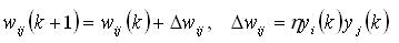
Initially, such a rule was applied to the McCulock-Pits threshold neurons, the output of which can be either 0 or 1, respectively. When applied to the threshold neuron formal model, the interpretation of Hebb's rule is closest to the original formulation.

However, since ordinary threshold neurons are rather inconvenient from the point of view of building INS for data processing ( although from a biological point of view they are probably the most realistic, but this is a completely different topic ), various modifications immediately appeared.

In the beginning, the most logical was to make the same threshold neuron, but with other possible outputs: -1 and 1. For quite a long time, this particular model of neuron was the most popular. However, let us see to what consequences the use of the formulation of the Hebbian rule indicated just above in the context of this model leads to. It is quite clear that this again leads to a split of the original rule. This is due to the fact that if the outputs of the pre- and postsynaptic neuron are different, then the second term in the weight adjustment formula takes a negative value, which means the initial value of the synaptic coefficient decreases (sometimes this effect is called the anti-hebbian rule ). As we could see earlier, there is no such mechanism in the original postulate of Hebb.

There are two reasons that I know of why such an assumption might seem acceptable to mathematicians. First, the application of the initial Hebbian rule leads to an unlimited increase in synaptic coefficients and, accordingly, to destabilization of the entire network as a whole. Secondly, in many earlier works [4], Hebb himself gave a similar mechanism by which the synaptic conductivity between two neurons decreases if the spikes of two neurons do not coincide. However, in formulating the final postulate, Chebb deliberately excluded such a mechanism.
In the future, the situation began to worsen, with the growing popularity of neuron models with a sigmoidal activation characteristic (Fig. 1). As we have seen earlier, the mathematical literature describes the use of the Hebbian rule in the case of training with a teacher. For the introduction of sigmoidal AH in terms of training with the teacher, Hebb's rule was modified and turned into a delta rule that is too far from any biological adequacy (that is why I will not discuss it in this article).


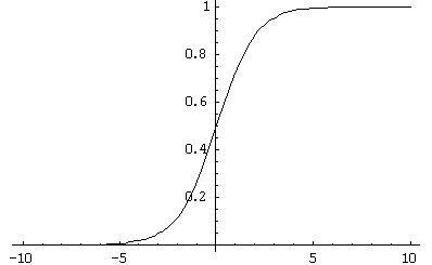
Fig. 1. Example of sigmoid activation function

However, in the case of self-study of the modification of the Hebbian rule, no one did and its application to threshold neurons with the outputs {-1; 1} leads to quite serious consequences. Indeed, since the sigmoid function is continuous, in most cases the output of the neuron is not zero. Thus, firstly, learning using the traditional Hebb's rule happens almost always, and secondly, the learning dynamics are now directly proportional to the values ​​of the outputs of the neurons (since they are continuous from 0 to 1 in absolute value). The latter is a fairly strong assumption, which from a neurophysiological point of view, to my knowledge, no one has ever tested. Despite this, in the technical tasks this technique gives the result, so everyone closed their eyes to this. However, if we formulate the Hebbian rule according to the original formulation for a sigmoidal neuron, then the following should result:


Of course, in the future, with the advent of spike neurons and the generalized STDP rule, the situation improved a little, but even at the moment, very few specialists use the spike neuron model. Therefore, a fundamental change in the situation can not be said.

Hebb's rule and training

Perhaps many of you will think about the name paradox, because the Hebbian rule is learning, but the title of the title was not chosen by chance. In the previous sections, we reviewed the history and origins of Hebb's postulate and several different misconceptions, which led to an incorrect interpretation of this rule. Now we will look at the initial neurophysiological postulate itself from the point of view of its applicability in bionic AI systems (and, accordingly, how likely is its leading role in animal / human learning processes).

Next, I will formulate three considerations , the essence of which will be reduced, at least, to my great doubts about the possibility of building self-learning systems based on Hebb's rule (or any modifications of it, of which there are an incredible amount). All considerations will be based on an analysis of hypothetical situations, with the third of them the least formalized, and the second - the most significant.

Consideration 1. Strengthening causality
If we disassemble the Hebb's rule from the point of view of a mathematician, then his action actually comes down to one operation: strengthening the causal connection. It turns out that initially this causal relationship should already be observed, i.e. first, neurons must be synaptically connected, and second, neurons must be synchronized (that is, a sequence must be observed — the spike on the presynaptic neuron -> the spike on the postsynaptic neuron ).

Imagine a hypothetical situation when, being in some kind of external environment, an agent / animal learned, using the Hebb's rule, to solve a certain problem that leads to an adaptive result. This means that the synaptic conductivity of the pathways of excitation between causal neurons has improved (the formulation itself makes me shiver, because then I will show where her legs grow from). Let us throw aside the initial proof of the possibility of learning, using only Hebb's rule, and since in fact we are going by contradiction, we take this situation as a starting point.

Now suppose that the environment has changed somewhat (the most common situation in real life) and our agent / animal cannot achieve an adaptive result in the way learned earlier. This means that the agent needs some retraining or additional education. At the same time, synaptic conductance is configured in such a way that it is easy to carry out the learned behavior. Re-training in such a situation is rather difficult, since despite the changed situation, the trained neurons will be activated along the chain, and despite everything, the previous behavior that does not lead to the achievement of the result will be implemented.

Consideration 2. Loss of acquired knowledge
Assume that learning by changing synaptic conductance can still occur. But then such training inevitably leads to loss of information (previously received information about the environment), which is distributed throughout the network. It is easy to understand if we imagine that the space of weighting factors is a field in which all the “knowledge” of the network is stored, and therefore changing this field, we do not add new “knowledge”, but overwrite all accumulated.

Since this is the most important consideration, a more detailed example should be given. As such, I will look at the behavior of the DARWIN robot [5], developed in the laboratory of Gerald Edelman, in the so-called Morris labyrinth .

Studies of the behavior of a mouse or rat in the Morris maze is one of the canonical biological experiments, which consists of the following. There is a pool with an opaque liquid (for example, it may be water tinted with milk), on the sides of the pool there are drawings that the mouse sees and can use for orientation. In a certain place of the pool there is a hidden platform that the mouse can find and thus escape - not to drown. The mouse is thrown into the pool, it swims for some time and either finds a platform and escapes, or starts to sink (then the experimenter saves it). After a series of experiments, the mouse begins to use landmarks on the sides of the pool and find the platform in a relatively short time. A schematic representation of such a labyrinth is shown in Fig. 2


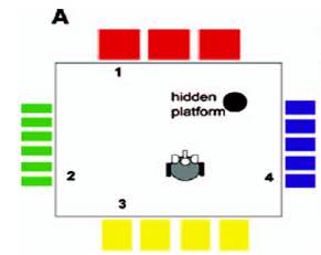
Fig. 2. Schematic image of the maze of Moriss

The DARWIN robot itself is quite complex - it simulates several real brain regions and their connections, in addition to several original structures (the control neural network in total has 90,000 neurons). Now it is important for us to know that the training of the robot is due to the specially modified Hebbian rule.

The robot is placed in the maze of Morissa and learns to find the platform, focusing on the drawings on the sides. At the same time, as a result, DARWIN quickly and effectively learns to find a platform. For further discussion, we will need to present a chain of such experiments.

Suppose a robot has learned to efficiently find a platform. Let's call this learning process - experiment 1 . Now move the platform somewhere else and again place the robot in the Morris maze (this will be experiment 2 ). At some point, the robot will become "clear" that the platform has moved and it will start searching again. Recalling that at the beginning of the discussion of this consideration, we temporarily accepted the postulate that retraining at the expense of Hebb's rule is fundamentally possible, we assume that the robot and in experiment 2 proved to be great and again learned how to effectively find the platform.

The most interesting thing begins when we try to conduct experiment 3 , once again moving the platform somewhere. In this case, the situation will be similar to experiment 2 - the robot will again understand that the platform has moved and will find its new position. It seems to be all right, but the most important in this case is the decision process. In the case of DARWIN, the solution process in Experiment 2 and Experiment 3 will be completely analogous. The robot will not even remember that they acquired some knowledge in experiment 1 , since they are no longer there - they were overwritten in the process of experiment 2 .

In the case of a real animal, the situation with the solution process in experiment 3 is completely different. In the beginning, it is clear that the animal will begin to look for a platform in the place that she learned in experiment 2 . However, not finding her there, she first checks the place where the platform was in experiment 1 . This most important feature is extremely adaptive in so many situations that the animal encounters during its life. By the way, a similar test with respect to the DARWIN system was invented not by me, but by my supervisor.

The loss of acquired knowledge is an inevitable consequence of any modifications of Hebb's rule.

Consideration 3. Hebb's Rule Reflex Nature
At its core, the Hebba rule is a reactivity postulate. Its application translates into a simplified sequential activation of the neuron chain. This is very similar to the concept of a reflex arc and learning, based on training this arc and facilitating the passage of a signal through it. At the same time, similar conclusions came to Kant in his time in his notes, which directly related to the ability of the human mind to learn.

From my point of view, it is very doubtful that the application of the Hebbian rule (I want to clarify that if only the Hebbian rule is applied) can lead to targeted training and ultimately achieve an adaptive result.The concept of purposeful is absent in the rule, as well as in any of its analyzes that I have seen.

Given the fact that a clear understanding of the fact that the brain (and each neuron) is an active rather than a reactive entity comes to us, a revision of the role of Hebb's postulate in teaching animals and humans is inevitable.

What to do?

What is the way out of this situation, you ask?

My answer will be the need to develop completely new approaches to learning modeling. At the moment, the Hebba rule and its numerous modifications are essentially the only biologically adequate learning / self-learning models. Of course, this is not accidental, since the neurophysiological postulate advanced by Hebb has a solid biological basis.

With all my criticism of Hebb's postulate, I did not mean to say that we do not observe it in the brain of animals. We observe of course and many famous works are devoted to this. I just wanted to turn your critical view on the role of this postulate in training.

I adhere to the position that the change in synaptic conduction is certainly one of the main factors ensuring effective training. However, this process and the postulate of Hebb are controlled by much more complex factors — the systemic level of brain organization . At the same time, the postulate itself is only a limited consequence of the entire set of system-level mechanisms.

Conclusion

In this review, we went from the history of Hebb's postulate to assess its capabilities and prospects for the implementation of training. I tried to draw your attention to some of the problems that arise if we put the mechanisms of Hebb's rule at the center of the training.

I repeat, now, more than ever, we have come up against the urgent need to formulate completely different, more complex, adaptive (targeted) learning mechanisms. How this one, conventionally called systemic, works today, we don’t know, there are only hypotheses. How the system level is provided by changing the synaptic conductivity and changes in the neurons themselves is an even more complex question, the answer to which we may not get soon. That is why, at the moment, specialists in the field of bionic AI need to introduce more abstract rules (while still operating directly with neurons and synapses), which will simulate the system mechanisms of learning, memory, decision making.

Bibliography

[1] . Hebb, DO The organization of behavior: a neuropsychological theory . New York (2002) ( Original edition - 1949 )
[2] . Rosenblatt F. Principles of Neurodynamics: Perceptrons and the Theory of Brain Mechanisms. Washington, DC: Spartan Books (1962).
[3] . Osovsky S. Neural networks for information processing (2002)
[4] . Hebb, DO Conditioned and unconditioned reflexes and inhibition . Unpublished MA Thesis, McGill University, Montreal, Quebec, (1932)
[5] . Krichmar JL, Seth AK, Nitz DA, Fleischer JG, Edelman GM «Spatial navigation and
causal analysis of a brain-based device modeling cortical-hippocampal interactions. ” Neuroinformatics , 2005. V. 3. No. 3. PP. 197-221.