Vehicle control via neural network

annotation

Using a neural network, we want the vehicle to drive itself, avoiding obstacles. We achieve this by choosing the appropriate I / O and careful training of the neural network. We feed the network distance to the nearest obstacles around the car, mimicking the vision of a human driver. At the output we get the acceleration and turn of the steering wheel of the vehicle. We also need to train the network on a variety of I / O strategies. The result is impressive even with just a few neurons! The car travels around obstacles, but it is possible to make some modifications so that this software can cope with more specific tasks.

Introduction

The idea is to have a vehicle that drives itself and avoids obstacles in the virtual world. Every moment it decides for itself how to change its speed and direction depending on the environment. In order to make it more real, the AI ​​should only see what the person would see if he were driving, so the AI ​​will only make decisions based on the obstacles that are in front of the vehicle. With realistic input, the AI ​​could be used in a real car and worked just as well.
When I hear the phrase: "Driving a vehicle using AI", I immediately think about computer games. Many of the racing games can use this technique to control vehicles, but there are a number of other applications that are looking for a means of managing vehicles in the virtual or real world.
So how are we going to do this? There are many ways to implement AI, but after all, if we need a “brain” to control a vehicle, then neural networks will fit perfectly. Neural networks work the same way as our brains. They will probably be the right choice. We must determine what will be the input and what will be the output of our neural network.

Neural networks

Neural networks appeared when studying the structure of the brain. Our brain consists of 10 ¹¹ neuron cells that send electrical signals to each other. Each neuron consists of one or two axons, which "produce a result", and a large number of dendrites, which receive input electrical signals. A neuron needs a certain input signal strength, which is added from all dendrites in order to be activated. After activation, the neuron sends an electrical signal down its axon to other neurons. Connections (axons and dendrites) are strengthened if they are often used.
This principle is applied in neural networks of smaller scales. Modern computers do not have the computing power that creates twenty billion neurons, but even with several neurons, the neural network can give a reasonable answer.
Neurons are organized into layers, as shown in Figure 1 . The input layer will have inputs, and depending on the strength of the connection with each neuron in the next layer, the input signal is fed to the next level. The strength of the joint is called weight. The value of each neuron in each layer will depend on the weight of the connection and the value of the neurons of the previous layer.

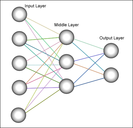
Picture 1
The driver can be compared with the "function". There are many inputs: what the driver sees. This data is processed by the brain as a function, and the reaction of the driver is the way out of the function.
The function f (x) = y converts the value x (one dimension) to y (one dimension).
We use the neural network of reverse propagation for the driver's “brain”, since such neural networks are able to approximate any function with areas of definition and values ​​that can have several dimensions: F (x1, x2, ..., xn) = y1, y2, ... yn .
This is exactly what we need, since we have to work with multiple inputs and outputs.
When a neural network consists of only a few neurons, we can calculate the weights necessary to obtain an acceptable result. But as the number of neurons increases, so does the complexity of the calculations. The back distribution network can be trained to establish the necessary weights. We just have to provide the desired results with the corresponding inputs.
After training, the neural network will respond to produce a result close to what you want when giving a known result, and to “guess” the correct answer at any input not corresponding to the trainer.
Actual calculations are beyond the scope of this article. There are many good books explaining how networks work with back-propagation errors.
The neural network used in this case has 4 layers ( Fig. 2 ). I tried various combinations of three to six layers. Everything worked perfectly with the three layers, but when I was teaching the network on a set of twenty-two inputs-outputs, the function approximation was not accurate enough. Five and six layers performed their task perfectly, but I had to spend considerable time on training (from 20 to 30 minutes on PII), and when I ran the program, it took a lot of processor time to perform the calculations.
In this network there are three neurons in the input layer and two in the resulting layer. Later I will explain why. Between them are two layers of eight neurons each. Again, I tested a layer with a larger and smaller number of neurons and stopped at eight, since this number gives an acceptable result.
When choosing the number of neurons, keep in mind that each layer and each neuron added to the system will increase the time required to calculate the weights.

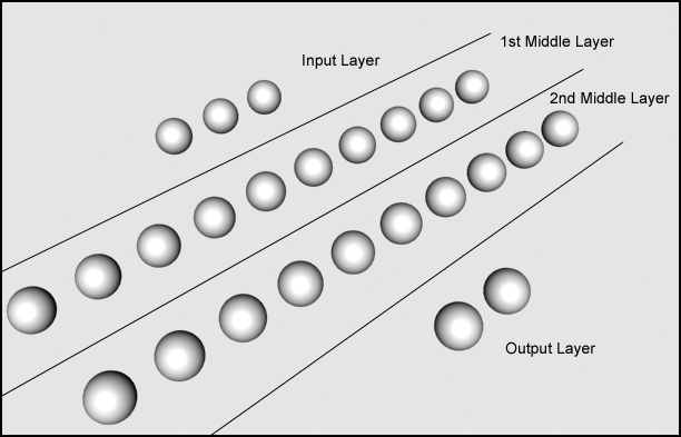
Figure 2
Adding neurons:
We have an input layer I with i neurons, and the resulting layer O with o neurons. We want to add one neuron to the middle layer M. The number of connections between neurons that we add is (i + o) .
Adding layers:
We have an input layer I with i neurons, and the resulting layer O with o neurons. We want to add M layers with m neurons in each. The number of connections between neurons that we add is (m * (i + o)) .
Now that we have looked at how the brain works, we need to understand how to determine the inputs and outputs of a neural network. The neural network itself does nothing if we give it information from the virtual world and do not respond to the network controller of the vehicle.

entrance

What information is important for driving? First, we must know the position of the obstacle towards us. Is this position to the right, to our left, or in front of us? If there are buildings on either side of the road, but there is nothing ahead, we accelerate. But if the car stopped in front of us, we slow down. Secondly, we need to know the distance from our position to the object. If the object is far away, we will continue to move until it approaches, and in this case, we slow down or stop.
This is exactly the information that we will use for our neural network. For simplicity, we introduce three relative directions: left, front, and right. As well as the distance from the obstacle to the vehicle.

Figure 3
We define the field of view of our AI driver and compile a list of objects that he sees. For simplicity, we use a circle in our example, but we could use a real cone truncated by six intersecting planes. Now for each object in this circle, we check if it is in the left field of view, right, or in the center.
At the entrance to the neural network is an array: float Vision [3] . The distances to the nearest obstacle to the left, in the center, and to the right of the vehicle will be stored in Vision [0] , Vision [1] and Vision [2], respectively. Figure 3 shows how this array looks like. The obstacle on the left is at a distance of 80% of the maximum distance, on the right - by 40%, and there are no obstacles in the center.
In order to calculate this, we need the position (x, y) of each object, the position (x, y) of the vehicle and the angle of the vehicle. We also need r (radius of the circle) and d _right , d _left - the vectors between the car and the L _right and L _left lines. These lines are parallel to the direction of movement of the car. Both vectors are perpendicular to the lines.
Although this is a 3D world, all math is two-dimensional, since the car cannot move in the third dimension, because it does not fly. All equations include only x and y , but not z .
First, we calculate the equations for the L _right and L _left lines to help us determine if an obstacle is to the right, left, or center of the vehicle.
Figure 4 is an illustration of all calculations.

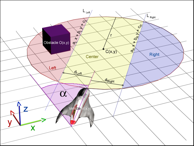
Figure 4

Where

Then we calculate the coordinates of a point on the line.

where V _x and V _y position of the vehicle.
Now we can finally calculate c _r

Similarly, we find the equation of the line L _left using the vector d _left .
Next, we must calculate the center of the circle. Everything inside the circle will be visible AI. The center of the circle C (x, y) at a distance r from the position of the car V (x, y) .


where V _x , V _{y is the} position of the vehicle and C _x , C _y is the center of the circle.
Then we check if each object in the world is within a circle (if the objects are organized into a quad tree or an octree tree, this process is much faster than a linked list).
If a 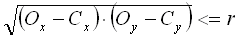, then the object is in a circle, where O _x , O _{y are the} coordinates of the obstacle.
For each object within a circle, we must check whether it is to the right, left, or center of the vehicle.
If a then the object is on the right side of the circle
otherwise if then the left side
otherwise in the center.
Calculate the distance from the object to the car

Now we store the distance in the corresponding part of the array ( Vision [0] , Vision [1] or Vision [2] ), provided that the previously stored distance is greater than the one just calculated. Initially, the Vision array must be initialized with the values 2r .
After checking each object, we have an array of Vision with distances to the nearest objects to the right, center and left of the car. If no object was found in this field of view, the array element will have a default value. , which means: "there is no object within sight."
Since the neural network uses the sigmoid function, the input data must be in the range from 0.0 to 1.0 . 0.0 will mean that the object touches the vehicle and 1.0 means that there are no objects within sight. Since we have set the maximum distance at which the AI ​​driver can see, we can easily bring all distances to a range from 0.0 to 1.0 .

')

Output

At the exit, we should receive instructions on how to change the vehicle speed and direction. It can be acceleration, braking and steering wheel angle. So we need two choices; one will be the acceleration / deceleration value (braking is just a negative acceleration), and the other will indicate a change in direction.
The result is between 0.0 and 1.0 for the same reason as the input. For acceleration, 0.0 means "full brake"; 1.0 is full throttle and 0.5 is no braking or acceleration. For steering, 0.0 means “all the way to the left,” 1.0 means “all the way to the right,” and 0.5 means not to change direction. So we need to translate the results into values ​​that we can use.


It should be noted that "negative acceleration" means braking if the vehicle moves forward, but it also means moving in the opposite direction if the car is at rest. In addition, "positive acceleration" means braking if the vehicle moves in the opposite direction.

Training

As I mentioned earlier, we first need to train a neural network. We need to create a set of inputs and their corresponding outputs.
Choosing the right I / O for training a neural network is probably the hardest part of the job. I had to train a network with a lot of data, watch how the car acted in the environment, and then change the records as needed. Depending on how we train the network, the vehicle may “fluctuate” in some situations and be immobilized.
We make a table ( Table 1 ) of the different position of the obstacles relative to the vehicle and the desired response of the AI.
Table 1

Input neurons Relative distance to the obstacle			Output neurons
Left	Centered	On right	Acceleration	Direction
No obstacles	No obstacles	No obstacles	Full throttle	Straight
Half way	No obstacles	No obstacles	Slight acceleration	Little to the right
No obstacles	No obstacles	Half way	Slight acceleration	Little left
No obstacles	Half way	No obstacles	Braking	Little left
Half way	No obstacles	Half way	Acceleration	Straight
Touching an object	Touching an object	Touching an object	Reverse	To the left
Half way	Half way	Half way	Without changes	Little left
Touching an object	No obstacles	No obstacles	Braking	Full right
No obstacles	No obstacles	Touching an object	Braking	Full left
No obstacles	Touching an object	No obstacles	Reverse	To the left
Touching an object	No obstacles	Touching an object	Full throttle	Straight
Touching an object	Touching an object	No obstacles	Reverse	Full right
No obstacles	Touching an object	Touching an object	Reverse	Full left
Object close	Object close	The object is very close	Without changes	To the left
The object is very close	Object close	Object close	Without changes	To the right
Touching an object	The object is very close	The object is very close	Braking	Full right
The object is very close	The object is very close	Touching an object	Braking	Full left
Touching an object	Object Close	Object Far	Without changes	To the right
Object away	Object close	Touching an object	Without changes	To the left
The object is very close	Object close	Object closer than halfway	Without changes	Full right
Object closer than halfway	Object close	The object is very close	Braking	Full left

And now you can translate it into numbers in table 2 .
table 2

Input neurons			Output neurons
Left	Centered	On right	Acceleration	Direction
1.0	1.0	1.0	1.0	0.5
0.5	1.0	1.0	0.6	0.7
1.0	1.0	0.5	0.6	0.3
1.0	0.5	1.0	0.3	0.4
0.5	1.0	0.5	0.7	0.5
0.0	0.0	0.0	0.2	0.2
0.5	0.5	0.5	0.5	0.4
0.0	1.0	1.0	0.4	0.9
1.0	1.0	0.0	0.4	0.1
1.0	0.0	1.0	0.2	0.2
0.0	1.0	0.0	1.0	0.5
0.0	0.0	1.0	0.3	0.8
1.0	0.0	0.0	0.3	0.2
0.3	0.4	0.1	0.5	0.3
0.1	0.4	0.3	0.5	0.7
0.0	0.1	0.2	0.3	0.9
0.2	0.1	0.0	0.3	0.1
0.0	0.3	0.6	0.5	0.8
0.6	0.3	0.0	0.5	0.2
0.2	0.3	0.4	0.5	0.9
0.4	0.3	0.2	0.4	0.1

Entrance:
0.0: The object almost touches the vehicle.
1.0: Object at the maximum distance from the vehicle or not an object in sight
Output:
Acceleration
0.0: Maximum negative acceleration (braking or vice versa)
1.0: Maximum Positive Acceleration
Direction
0,0: Complete left turn
0.5: Straight
1.0: Turn right

Conclusion / Ways to Improve

The use of a neural network back propagation is suitable for our purposes, but there are some problems identified during testing. Some changes could make the program more reliable and adapt it to other situations. Now I will describe to you some problems that you might want to think about.

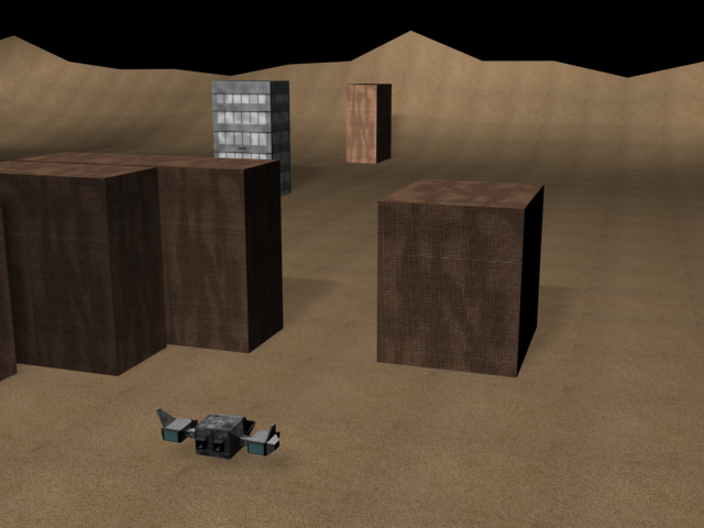
Figure 5
The vehicle is “stuck” for a while, as it fluctuates in deciding whether to drive left or right. This was to be expected: people sometimes have the same problem. To fix this is not so easy, trying to adjust the weights of the neural network. But we can add a line of code that says:
"If (the vehicle does not move for 5 seconds), then (take control and turn it 90 degrees to the right)."
By this we can guarantee that the car will never stand still, not knowing what to do.
The vehicle will not see a small gap between the two houses, as shown in Figure 5 . Since we do not have a high level of accuracy in vision (on the left, in the center, on the right), two buildings that are close to each other will be like a wall for artificial intelligence. To have a clearer view of our AI, we need to have 5 or 7 levels of accuracy at the entrance to the neural network. Instead of "right, center, left," we could have "far right, right side, center, side left, far left." With a good learning of the neural network, artificial intelligence will see the gap and understand that it can pass through it.
It works in a 2D world, but what if the vehicle is able to fly through a cave? With some changes to this technique, we can make the AI ​​fly, not ride. By analogy with the last problem, we increase the accuracy of the gaze. But instead of adding “rights” and “lion”, we can do it as shown in table 3 .
Table 3

Top left	Up	Top right
Left	Centre	On right
Bottom left	Down below	Bottom right

Now that our neural network can see the world in 3D, we just need to change our vehicle control and response to the world.
The vehicle only "wanders" without any specific purpose. It does nothing but circumvent obstacles. Depending on where we want to go, we can “tune” the brain as needed. We can have many different neural networks and use the right one in a particular situation. For example, we could follow the car in sight. We just need to connect another neural network trained to follow another vehicle, receiving as input the location of the second transport.
As we have just seen, this method can be improved and applied in various fields. Even if it is not used for any useful purpose, it will still be interesting for us to observe how the artificial intelligence system behaves in the environment. If you observe for a long time, we will understand that in difficult conditions, the vehicle will not always follow the same path due to the small difference in the decision due to the nature of the neural network. The car will sometimes drive to the left of the building, and sometimes to the right of the same building.

Literature

1. Joey Rogers, Object-Oriented Neural Network in C ++, Academic Press, San Diego, CA, 1997
2. MT Hagan, HB Demuth and MH Beale, Neural Network Design, PWS Publishing, Boston, MA, 1995