Pedestrian detection is mainly used in research on unmanned vehicles. The general purpose of detecting pedestrians is to prevent a car from colliding with a person. On Habré recently there was a topic about " smart machines ". The creation of such systems is a very popular area of ​​research ( Darpa challenge ). I am engaged in the recognition of pedestrians for a similar project of intelligent cars. Obviously, the problem of detecting pedestrians is software, and collision avoidance is hardware. In this article I will only mention the program part, briefly describe one method of detecting people in an image and a classification algorithm.

Introduction

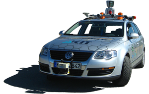
In my work I use two sensors: an infrared camera and a lidar . The temperature of the human body is usually above the environment. Therefore, the image from the infrared camera of a person can be easily localized. As a rule, it is easy to detect the unclosed parts of the body: the head and hands. But with the help of the camera alone it is difficult to determine the size of the object, it is difficult to say how far a person is from the camera. This is where a lidar comes in. It measures the distance to objects.

Why do we need a lidar? Let's look at our pictures for a start. The whole idea of ​​preprocessing an image comes down to localizing areas of interest. We do not care what the whole image is. We want to highlight several areas and work further with them. Ideally, the area of ​​interest should encompass images of a person entirely. Knowing that the head of a person is warmer than the environment, we easily find it in the image. Next we need to estimate the size of a person. This is where the data from the lidar come to the rescue. Knowing the distance to the object, the focal length of the camera, the size of the object in the coordinates of the real world, it is easy to calculate the size of the object in pixels. We determined the size of the object in real-world coordinates equal to a 2 by 1 meter rectangle in the confidence that the average person fits into such a rectangle. But in the coordinate system, the images of the region of interest are still of different sizes. Another scale transformation and finally all areas of interest not only cover the same area of ​​the real world, but also have the same dimensions in pixels.

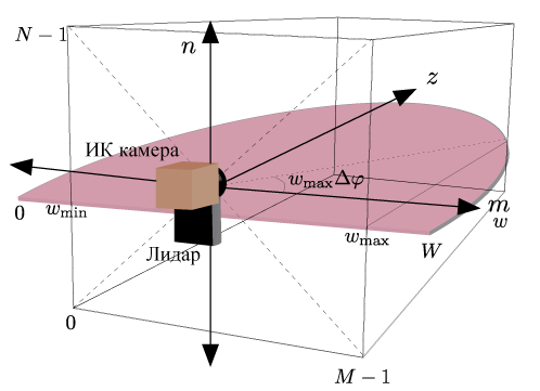
Let us consider how to combine the data of two sensors: we find the hot area in the image (we assume that this is the human head), calculate the angle at which the center of this area is located, we reduce this angle to the lidar coordinate system and get the distance to the object from this angle. To transfer the angle from one coordinate system to another, the sensors must be calibrated. Instead of the present calibration of sensors, their specific location is used, at which the centers of the sensors coincide in the horizontal plane:

')
Of course, on a test machine, things are a little different. First, the figure below shows the location of static sensors: their position does not change with time. Secondly, our test machine uses a different type of lidar - three-dimensional. It is installed in the middle of the roof of the car. The camera is installed in front of the roof. Thus, the centers of the sensors can no longer be considered to be at one point. I see two options for solving this problem: in parallel, transfer data from the coordinate system of one sensor to the coordinate system of another sensor (after measuring the distance between them), or (automatically) calibrate the sensors.

Extracting areas of interest

Extracting features that are used for pattern recognition, and their classification takes a lot of time. Processing one frame with 6–7 objects in Matlab can take a full minute. For real-time oriented systems, such long processing is unacceptable. The speed is strongly influenced by the number of warm objects detected, and the person is not the only warm object. Parts of cars, windows, traffic lights can also stand out against the general temperature background. In this paper, the emphasis is on the speed of information processing. We need to quickly weed out a maximum of objects that are definitely not human. It is advisable not to miss a single real person. All remaining objects can then be classified using the full static classifier.

Hot areas in the image are detected using a method called “Maximum Stable Extreme Areas” (MCPU from the English. Maximally Stable Extremal Regions [1]). The original image is processed by a threshold function with a variable threshold value. The result is a new image sequence, the size of which corresponds to the number of different threshold values ​​(for example, for a monochrome image with pixel values ​​from 0 to 255, we obtain 256 images). The first image in the sequence will be completely white. Black areas will appear next and the latest image in the sequence will be completely black. The figure below shows this sequence in the form of animation:


The white areas in the image are areas of extremum. We can analyze how long this or that area of ​​extremum is present in the sequence of images. To do this, you can use another threshold function. For example, with a value of 10. If an extremum region is present on more than 10 sequence images, then this region is called the most stable extremum region.

Having found the most stable areas of interest, we can filter them a little more: check the aspect ratio, discard objects far from the camera, process the overlapping areas.

Source image	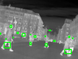Maximum stable extremum areas
Areas of interest	Filtered areas of interest

Dispersion

As a metric for the classification of objects used "dispersion" [2]. The calculation of this metric takes little time and, moreover, its value is invariant to the lighting conditions. It is considered according to the formula . In the original paper, the variance is calculated by the contour of the object. To obtain the contour from the areas of interest, the Gauss filter and the Sobel operator are applied successively. The decision on whether an image belongs to a particular class is made using a threshold function. Images of people have a lower dispersion value than images of machine parts or buildings.

Conclusion

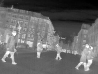
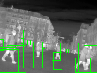
The results of the algorithm in pictures:


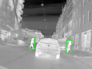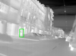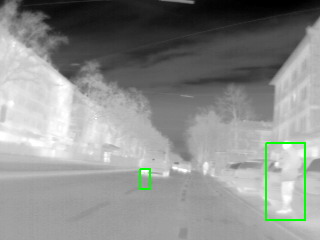The test computer is equipped with an Intel Core 2 Duo processor with a frequency of 3 GHz, 6 MB cache, 2 GB RAM. Tests were conducted in the system Matlab. The average processing time per frame is 64 ms. This means that in 1 second the system will be able to process approximately 16 frames. This, of course, is better than 1 frame per minute.

The following questions naturally arise: how reliable is the variance for classification, how will the time spent working on one frame increase when using a full-fledged classifier. I have no answers to these questions yet. Now I am working on it. There will be results - I will inform you!

Literature

[1] J. Matas, O. Chum, M. Urban, and T. Pajdla, “Robust wide baseline stereo from maximally stable extremal regions,” in British Machine Vision Conference, 2002, pp. 384–396.
[2] AL Hironobu, AJ Lipton, H. Fujiyoshi, and RS Patil, “Moving Target Classification and Tracking From Real-Time Video,” in Applications of Computer Vision, 1998. WACV '98. Proceedings., Fourth IEEE Workshop on, October 1998, pp. 8–14.